The SVM Optimization Problem

---

SVMs search for the optimal hyperplane

The Perceptron has several advantages: it is a simple model, the algorithm is very easy to implement, and we have a theoretical proof that it will find a hyperplane that separates the data. However, its biggest weakness is that it will not find the same hyperplane every time. Why do we care? Because not all separating hyperplanes are equals. If the Perceptron gives you a hyperplane that is very close to all the data points from one class, you have a right to believe that it will generalize poorly when given new data.

SVMs do not have this problem. Indeed, instead of looking for a hyperplane, SVMs tries to find the hyperplane. We will call this the optimal hyperplane, and we will say that it is the one that best separates the data.

How can we compare two hyperplanes?

Because we cannot choose the optimal hyperplane based on our feelings, we need some sort of metric that will allow us to compare two hyperplanes and say which one is superior to all others.

In this section, we will try to discover how we can compare two hyperplanes. In other words, we will search for a way to compute a number that allows us to tell which hyperplane separates the data the best. We will look at methods that seem to work, but then we will see why they do not work and how we can correct their limitations. Let us try with a simple attempt to compare two hyperplanes using only the equation of the hyperplane.

Using the equation of the hyperplane

Given an example and a hyperplane, we wish to know how the example relates to the hyperplane.

One key element we already know is that if the value of satisfies the equation of a line, then it means it is on the line. It works in the same way for a hyperplane: for a data point and a hyperplane defined by a vector and bias , we will get    if is on the hyperplane.

But what if the point is not on the hyperplane?

Let us see what happens with an example. In Figure 22, the line is defined by  and . When we use the equation of the hyperplane:

• for point , using vector   we get  
• for point , using vector   we get  
• for point , using vector   we get  

Figure 22: The equation returns a bigger number for A than for B

As you can see, when the point is not on the hyperplane we get a number different from zero. In fact, if we use a point far away from the hyperplane, we will get a bigger number than if we use a point closer to the hyperplane.

Another thing to notice is that the sign of the number returned by the equation tells us where the point stands with respect to the line. Using the equation of the line displayed in Figure 23, we get:

• for point
• for point
• for point

Figure 23: The equation returns a negative number for C

If the equation returns a positive number, the point is below the line, while if it is a negative number, it is above. Note that it is not necessarily visually above or below, because if you have a line like the one in Figure 24, it will be left or right, but the same logic applies. The sign of the number returned by the equation of the hyperplane allows us to tell if two points lie on the same side. In fact, this is exactly what the hypothesis function we defined in Chapter 2 does.

Figure 24: A line can separate the space in different ways

We now have the beginning of a solution for comparing two hyperplanes.

Given a training example and a hyperplane defined by a vector and bias , we compute the number   to know how far the point is from the hyperplane.

Given a data set , we compute   for each training example, and say that the number is the smallest   we encounter.

If we need to choose between two hyperplanes, we will then select the one from which is the largest.

To be clear, this means that if we have hyperplanes, we will compute    and select the hyperplane having this .

Problem with examples on the negative side

Unfortunately, using the result of the hyperplane equation has its limitations. The problem is that taking the minimum value does not work for examples on the negative side (the ones for which the equation returns a negative value).

Remember that we always wish to take the of the point being the closest to the hyperplane. Computing with examples on the positive side actually does this. Between two points with    and  , we pick the one having the smallest number, so we choose . However, between two examples having and , this rule will pick   because   is smaller than , but the closest point is actually the one with .

One way to fix this problem is to consider the absolute value of .

Given a data set , we compute for each example and say that is the having the smallest absolute value:

Does the hyperplane correctly classify the data?

Computing the number allows us to select a hyperplane. However, using only this value, we might pick the wrong one. Consider the case in Figure 25: the examples are correctly classified, and the value of computed using the last formula is 2.

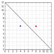
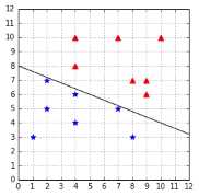
Figure 25: A hyperplane correctly classifying the data

In Figure 26, the examples are incorrectly classified, and the value of is also 2. This is problematic because using , we do not know which hyperplane is better. In theory, they look equally good, but in reality, we want to pick the one from Figure 25.

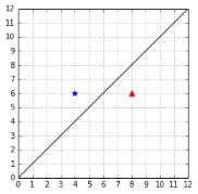
Figure 26: A hyperplane that does not classify the data correctly

How can we adjust our formula to meet this requirement?

Well, there is one component of our training example that we did not use: the !

If we multiply   by the value of , we change its sign. Let us call this new number :

The sign of will always be:

• Positive if the point is correctly classified
• Negative if the point is incorrectly classified

Given a data set , we can compute:

With this formula, when comparing two hyperplanes, we will still select the one for which is the largest. The added bonus is that in special cases like the ones in Figure 25 and Figure 26, we will always pick the hyperplane that classifies correctly (because will have a positive value, while its value will be negative for the other hyperplane).

In the literature, the number has a name, it is called the functional margin of an example; its value can be computed in Python, as shown in Code Listing 19. Similarly, the number is known as the functional margin of the data set .

Code Listing 19

Using this formula, we find that the functional margin of the hyperplane in Figure 25 is +2, while in Figure 26 it is -2. Because it has a bigger margin, we will select the first one.

Tip: Remember, we wish to choose the hyperplane with the largest margin.

Scale invariance

It looks like we found a good way to compare the two hyperplanes this time. However, there is a major problem with the functional margin: is not scale invariant.

Given a vector and bias , if we multiply them by 10, we get and . We say we rescaled them.

The vectors   and , represent the same hyperplane because they have the same unit vector. The hyperplane being a plane orthogonal to a vector , it does not matter how long the vector is. The only thing that matters is its direction, which, as we saw in the first chapter, is given by its unit vector. Moreover, when tracing the hyperplane on a graph, the coordinate of the intersection between the vertical axis and the hyperplane will be  , so the hyperplane does not change because of the rescaling of , either.

The problem, as we can see in Code Listing 20, is that when we compute the functional margin with , we get a number ten times bigger than with . This means that given any hyperplane, we can always find one that will have a larger functional margin, just by rescaling and .

Code Listing 20

To solve this problem, we only need to make a small adjustment. Instead of using the vector , we will use its unit vector. To do so, we will divide by its norm. In the same way, we will divide by the norm of to make it scale invariant as well.

Recall the formula of the functional margin: 

We modify it and obtain a new number :

 

As before, given a data set , we can compute:

The advantage of is that it gives us the same number no matter how large is the vector   that we choose. The number also has a name—it is called the geometric margin of a training example, while is the geometric margin of the dataset. A Python implementation is shown in Code Listing 21.

Code Listing 21

We can verify that the geometric margin behaves as expected. In Code Listing 22, the function returns the same value for the vector or its rescaled version .

Code Listing 22

It is called the geometric margin because we can retrieve this formula using simple geometry. It measures the distance between and the hyperplane.

In Figure 27, we see that the point is the orthogonal projection of into the hyperplane. We wish to find the distance between and .

Figure 27: The geometric margin is the distance d between the point X and the hyperplane

The vector has the same direction as the vector , so they share the same unit vector . We know that the norm of is , so the vector can be defined by  .

Moreover, we can see that , so if we substitute for and do a little bit of algebra, we get:

Now, the point is on the hyperplane. It means that satisfies the equation of the hyperplane, and we have:

Eventually, as we did before, we multiply by to ensure that we select a hyperplane that correctly classifies the data, and it gives us the geometric margin formula we saw earlier:

Now that we have defined the geometric margin, let us see how it allows us to compare two hyperplanes. We can see that the hyperplane in Figure 28 is closer to the blue star examples than to the red triangle examples as compared to the one in Figure 29. As a result, we expect its geometric margin to be smaller. Code Listing 23 uses the function defined in Code Listing 21 to compute the geometric margin for each hyperplane. As expected from Figure 29, the geometric margin of the second hyperplane defined by and   is larger (0.64 > 0.18). Between the two, we would select this hyperplane.

Code Listing 23

We see that to compute the geometric margin for another hyperplane, we just need to modify the value of or . We could try to change it by a small increment to see if the margin gets larger, but it is kind of random, and it would take a lot of time. Our objective is to find the optimal hyperplane for a dataset among all possible hyperplanes, and there is an infinity of hyperplanes.

Tip: Finding the optimal hyperplane is just a matter of finding the values of w and b for which we get the largest geometric margin.

How can we find the value of that produces the largest geometric margin? Luckily for us, mathematicians have designed tools to solve such problems. To find and , we need to solve what is called an optimization problem. Before looking at what the optimization problem is for SVMs, let us do a quick review of what an optimization problem is.

What is an optimization problem?

Unconstrained optimization problem

The goal of an optimization problem is to minimize or maximize a function with respect to some variable x (that is, to find the value of x for with the function returns its minimum or maximum value). For instance, the problem in which we want to find the minimum of the function   is written:

Or, alternatively:

In this case, we are free to search amongst all possible values of . We say that the problem is unconstrained. As we can see in Figure 30, the minimum of the function is zero at .

Constrained optimization problem

Single equality constraint

Sometimes we are not interested in the minimum of the function by itself, but rather its minimum when some constraints are met. In such cases, we write the problem and add the constraints preceded by  , which is often abbreviated  For instance, if we wish to know the minimum of but restrict the value of to a specific value, we can write:

This example is illustrated in Figure 31. In general, constraints are written by keeping zero on the right side of the equality so the problem can be rewritten:

Using this notation, we clearly see that the constraint is an affine function while the objective function is a quadratic function. Thus we call this problem a quadratic optimization problem or a Quadratic Programming (QP) problem.

Feasible set

The set of variables that satisfies the problem constraints is called the feasible set (or feasible region). When solving the optimization problem, the solution will be picked from the feasible set. In Figure 31, the feasible set contains only one value, so the problem is trivial. However, when we manipulate functions with several variables, such as , it allows us to know from which values we are trying to pick a minimum (or maximum).

For example:

In this problem, the feasible set is the set of all pairs of points , such as .

Multiple equality constraints and vector notation

We can add as many constraints as we want. Here is an example of a problem with three constraints for the function :

When we have several variables, we can switch to vector notation to improve readability. For the vector  the function becomes , and the problem is written:

When adding constraints, keep in mind that doing so reduces the feasible set. For a solution to be accepted, all constraints must be satisfied.

For instance, let us look at the following the problem: 

We could think that and are solutions, but this is not the case. When , the constraint is not met; and when , the constraint is not met. The problem is infeasible.

Tip: If you add too many constraints to a problem, it can become infeasible.

If you change an optimization problem by adding a constraint, you make the optimum worse, or, at best, you leave it unchanged (Gershwin, 2010).

Inequality constraints

We can also use inequalities as constraints:

And we can combine equality constraints and inequality constraints:

How do we solve an optimization problem?

Several methods exist that can solve each type of optimization problem. However, presenting them is outside the scope of this book. The interested reader can see Optimization Models and Application (El Ghaoui, 2015) and Convex Optimization (Boyd & Vandenberghe, 2004), two good books for starting on the subject and that are available online for free (see Bibliography for details). We will instead focus on the SVMs again and derive an optimization problem allowing us to find the optimal hyperplane. How to solve the SVMs optimization problem will be explained in detail in the next chapter.

The SVMs optimization problem

Given a linearly separable training set and a hyperplane with a normal vector and bias , recall that the geometric margin of the hyperplane is defined by:

where   is the geometric margin of a training example .

The optimal separating hyperplane is the hyperplane defined by the normal vector and bias for which the geometric margin is the largest.

To find and , we need to solve the following optimization problem, with the constraint that the margin of each example should be greater or equal to :

There is a relationship between the geometric margin and the functional margin:

So we can rewrite the problem:

We can then simplify the constraint by removing the norm on both sides of the inequality:

Recall that we are trying to maximize the geometric margin and that the scale of and does not matter. We can choose to rescale and as we want, and the geometric margin will not change. As a result, we decide to scale and so that . It will not affect the result of the optimization problem.

The problem becomes:

Because   it is the same as:

And because we decided to set , this is equivalent to:

This maximization problem is equivalent to the following minimization problem:

Tip: You can also read an alternate derivation of this optimization problem on this page, where I use geometry instead of the functional and geometric margins.

This minimization problem gives the same result as the following:

The factor has been added for later convenience, when we will use QP solver to solve the problem and squaring the norm has the advantage of removing the square root.

Eventually, here is the optimization problem as you will see it written in most of the literature:

Why did we take the pain of rewriting the problem like this? Because the original optimization problem was difficult to solve. Instead, we now have convex quadratic optimization problem, which, although not obvious, is much simpler to solve.

Summary

First, we assumed that some hyperplanes are better than others: they will perform better with unseen data. Among all possible hyperplanes, we decided to call the “best” hyperplane the optimal hyperplane. To find the optimal hyperplane, we searched for a way to compare two hyperplanes, and we ended up with a number allowing us to do so. We realized that this number also has a geometrical meaning and is called the geometric margin.

We then stated that the optimal hyperplane is the one with the largest geometric margin and that we can find it by maximizing the margin. To make things easier, we noted that we could minimize the norm of , the vector normal to the hyperplane, and we will be sure that it will be the of the optimal hyperplane (because if you recall, is used in the formula for computing the geometric margin).