Support Vector Machines Succinctly^®
by Alexandre Kowalczyk

CHAPTER 8

The SMO Algorithm

We saw how to solve the SVM optimization problem using a convex optimization package. However, in practice, we will use an algorithm specifically created to solve this problem quickly: the SMO (sequential minimal optimization) algorithm. Most machine learning libraries use the SMO algorithm or some variation.

The SMO algorithm will solve the following optimization problem:

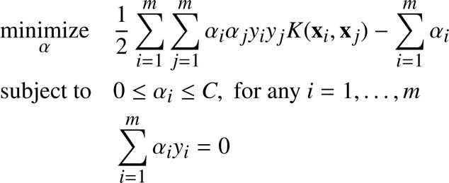
$%FontSize=11 %TeXFontSize=11 \documentclass{article} \pagestyle{empty} \begin{document} \begin{equation*} \begin{aligned} & \underset{\alpha}{\text{minimize}} & & \frac{1}{2}\sum\limits_{i=1}^m \sum\limits_{j=1}^m \alpha_i\alpha_j y_i y_j K(\mathbf{x}_i,\mathbf{x}_j) - \sum\limits_{i=1}^m \alpha_i \\ & \text{subject to} & & 0 \leq \alpha_i \leq C, \; \text{for any}\ i = 1, \ldots, m \\ & & & \sum\limits_{i=1}^m \alpha_i y_i=0 \\ \end{aligned} \end{equation*}\end{document}$

It is a kernelized version of the soft-margin formulation we saw in Chapter 5. The objective function we are trying to minimize can be written in Python (Code Listing 37):

Code Listing 37

def kernel(x1, x2):
return np.dot(x1, x2.T)

def objective_function_to_minimize(X, y, a, kernel):
    m, n = np.shape(X)
    return 1 / 2 * np.sum([a[i] * a[j] * y[i] * y[j]* kernel(X[i, :], X[j, :])
                           for j in range(m)
                           for i in range(m)])\
           - np.sum([a[i] for i in range(m)])

This is the same problem we solved using CVXOPT. Why do we need another method? Because we would like to be able to use SVMs with big datasets, and using convex optimization packages usually involves matrix operations that take a lot of time as the size of the matrix increases or become impossible because of memory limitations. The SMO algorithm has been created with the goal of being faster than other methods.

The idea behind SMO

When we try to solve the SVM optimization problem, we are free to change the values of $%FontSize=11 %TeXFontSize=11 \documentclass{article} \pagestyle{empty} \begin{document} \[ \alpha \] \end{document}$ as long as we respect the constraints. Our goal is to modify $%FontSize=11 %TeXFontSize=11 \documentclass{article} \pagestyle{empty} \begin{document} \[ \alpha \] \end{document}$ so that in the end, the objective function returns the smallest possible value. In this context, given a vector $%FontSize=11 %TeXFontSize=11 \documentclass{article} \pagestyle{empty} \begin{document} \[ \alpha = (\alpha_1, \alpha_2, \dots, \alpha_m) \] \end{document}$ of Lagrange multipliers, we can change the value of any $%FontSize=11 %TeXFontSize=11 \documentclass{article} \pagestyle{empty} \begin{document} \[ \alpha_i \] \end{document}$ until we reach our goal.

The idea behind SMO is quite easy: we will solve a simpler problem. That is, given a vector $%FontSize=11 %TeXFontSize=11 \documentclass{article} \pagestyle{empty} \begin{document} \[ \alpha = (\alpha_1, \alpha_2, \dots, \alpha_m) \] \end{document}$ , we will allow ourselves to change only two values of $%FontSize=11 %TeXFontSize=11 \documentclass{article} \pagestyle{empty} \begin{document} \[ \alpha \] \end{document}$ , for instance, $%FontSize=11 %TeXFontSize=11 \documentclass{article} \pagestyle{empty} \begin{document} \[ \alpha_3 \] \end{document}$ and $%FontSize=11 %TeXFontSize=11 \documentclass{article} \pagestyle{empty} \begin{document} \[ \alpha_7 \] \end{document}$ . We will change them until the objective function reaches its minimum given this set of alphas. Then we will pick two other alphas and change them until the function returns its smallest value, and so on. If we continue doing that, we will eventually reach the minimum of the objective function of the original problem.

SMO solves a sequence of several simpler optimization problems.

How did we get to SMO?

This idea of solving several simpler optimization problems is not new. In 1982, Vapnik proposed a method known as “chunking,” which breaks the original problem down into a series of smaller problems (Vapnik V. , 1982). What made things change is that in 1997, Osuna, et al., proved that solving a sequence of sub-problems will be guaranteed to converge as long as we add at least one example violating the KKT conditions (Osuna, Freund, & Girosi, 1997).

Using this result, one year later, in 1998, Platt proposed the SMO algorithm.

Why is SMO faster?

The great advantage of the SMO approach is that we do not need a QP solver to solve the problem for two Lagrange multipliers—it can be solved analytically. As a consequence, it does not need to store a huge matrix, which can cause problems with machine memory. Moreover, SMO uses several heuristics to speed up the computation.

The SMO algorithm

The SMO algorithm is composed of three parts:

One heuristic to choose the first Lagrange multiplier
One heuristic to choose the second Lagrange multiplier
The code to solve the optimization problem analytically for the two chosen multipliers

Tip: A Python implementation of the algorithm is available in Appendix B: The SMO Algorithm. All code listings in this section are taken from this appendix and do not work alone.

The analytical solution

At the beginning of the algorithm, we start with a vector in which $%FontSize=11 %TeXFontSize=11 \documentclass{article} \pagestyle{empty} \begin{document} \[ \alpha_i=0 \quad \text{for all}\ i = 1,\dots,m \] \end{document}$ . The idea is to pick two elements of this vector, which we will name $%FontSize=11 %TeXFontSize=11 \documentclass{article} \pagestyle{empty} \begin{document} \[ \alpha_1 \] \end{document}$ and $%FontSize=11 %TeXFontSize=11 \documentclass{article} \pagestyle{empty} \begin{document} \[ \alpha_2 \] \end{document}$ , and to change their values so that the constraints are still respected.

The first constraint $%FontSize=11 %TeXFontSize=11 \documentclass{article} \pagestyle{empty} \begin{document} \[ 0 \leq \alpha_i \leq C, \; \text{for any}\ i = 1, \ldots, m \] \end{document}$ means that $%FontSize=11 %TeXFontSize=11 \documentclass{article} \pagestyle{empty} \begin{document} \[ 0 \leq \alpha_1 \leq C \] \end{document}$ and $%FontSize=11 %TeXFontSize=11 \documentclass{article} \pagestyle{empty} \begin{document} \[ 0 \leq \alpha_2 \leq C \] \end{document}$ . That is why we are forced to select a value lying in the blue box of Figure 50 (which displays an example where $%FontSize=11 %TeXFontSize=11 \documentclass{article} \pagestyle{empty} \begin{document} \[ C=5 \] \end{document}$ ).

The second constraint is a linear constraint $%FontSize=11 %TeXFontSize=11 \documentclass{article} \pagestyle{empty} \begin{document} \[ \sum\limits_{i=1}^m \alpha_i y_i=0 \] \end{document}$ . It forces the values to lie on the red diagonal, and the first couple of selected $%FontSize=11 %TeXFontSize=11 \documentclass{article} \pagestyle{empty} \begin{document} \[ \alpha_1 \] \end{document}$ and $%FontSize=11 %TeXFontSize=11 \documentclass{article} \pagestyle{empty} \begin{document} \[ \alpha_2 \] \end{document}$ should have different labels ( $%FontSize=11 %TeXFontSize=11 \documentclass{article} \pagestyle{empty} \begin{document} \[ y_1 \neq y_2 \] \end{document}$ ).

The feasible set is the diagonal of the box

Figure 50: The feasible set is the diagonal of the box

In general, to avoid breaking the linear constraint, we must change the multipliers so that:

$%FontSize=11 %TeXFontSize=11 \documentclass{article} \pagestyle{empty} \begin{document} \[ \alpha_1 y_1 + \alpha_2 y2 = constant = \alpha_1^{old} y_1 + \alpha_2^{old} y2 \] \end{document}$

We will not go into the details of how the problem is solved analytically, as it is done very well in (Cristianini & Shawe-Taylor, 2000) and in (Platt J. C., 1998).

Remember that there is a formula to compute the new $%FontSize=11 %TeXFontSize=11 \documentclass{article} \pagestyle{empty} \begin{document} \[ \alpha_2 \] \end{document}$ :

$%FontSize=11 %TeXFontSize=11 \documentclass{article} \pagestyle{empty} \begin{document} \[ \alpha_2^{new} = \alpha_2 + \frac{y_2(E_1-E_2)}{K(\mathbf{x}_1,\mathbf{x}_1)+K(\mathbf{x}_2,\mathbf{x}_2)- 2 K(\mathbf{x}_1,\mathbf{x}_2)} \] \end{document}$

with $%FontSize=11 %TeXFontSize=11 \documentclass{article} \pagestyle{empty} \begin{document} \[ E_i = f(\mathbf x_i)-yi \] \end{document}$ being the difference between the output of the hypothesis function and the example label. $%FontSize=11 %TeXFontSize=11 \documentclass{article} \pagestyle{empty} \begin{document} \[ K \] \end{document}$ is the kernel function. We also compute bounds, which applies to $%FontSize=11 %TeXFontSize=11 \documentclass{article} \pagestyle{empty} \begin{document} \[ \alpha_2^{new} \] \end{document}$ ; it cannot be smaller than the lower bound, or larger than the upper bound, or constraints will be violated. So $%FontSize=11 %TeXFontSize=11 \documentclass{article} \pagestyle{empty} \begin{document} \[ \alpha_2^{new} \] \end{document}$ is clipped if this is the case.

Once we have this new value, we use it to compute the new $%FontSize=11 %TeXFontSize=11 \documentclass{article} \pagestyle{empty} \begin{document} \[ \alpha_1 \] \end{document}$ using this formula:

$%FontSize=11 %TeXFontSize=11 \documentclass{article} \pagestyle{empty} \begin{document} \[ \alpha_1^{new}= \alpha_1^{old}+y_1 y_2(\alpha_2^{old}-\alpha_2^{new}) \] \end{document}$

Understanding the first heuristic

The idea behind the first heuristic is pretty simple: each time SMO examines an example, it checks whether or not the KKT conditions are violated. Recall that at least one KKT condition must be violated. If the conditions are met, then it tries another example. So if there are millions of examples, and only a few of them violate the KKT conditions, it will spend a lot of time examining useless examples. In order to avoid that, the algorithm concentrates its time on examples in which the Lagrange multiplier is not equal to 0 or $%FontSize=11 %TeXFontSize=11 \documentclass{article} \pagestyle{empty} \begin{document} \[ C \] \end{document}$ , because they are the most likely to violate the conditions (Code Listing 38).

Code Listing 38

def get_non_bound_indexes(self):
    return np.where(np.logical_and(self.alphas > 0,
                                   self.alphas < self.C))[0]

# First heuristic: loop over examples where alpha is not 0 and not C
# they are the most likely to violate the KKT conditions
# (the non-bound subset).
def first_heuristic(self):
    num_changed = 0
    non_bound_idx = self.get_non_bound_indexes()

    for i in non_bound_idx:
        num_changed += self.examine_example(i)
    return num_changed

Because solving the problem analytically involves two Lagrange multipliers, it is possible that a bound multiplier (whose value is between 0 and $%FontSize=11 %TeXFontSize=11 \documentclass{article} \pagestyle{empty} \begin{document} \[ C \] \end{document}$ ) has become KKT-violated. That is why the main routine alternates between all examples and the non-bound subset (Code Listing 39). Note that the algorithm finishes when progress is no longer made.

Code Listing 39

def main_routine(self):
    num_changed = 0
    examine_all = True

    while num_changed > 0 or examine_all:
        num_changed = 0

        if examine_all:
            for i in range(self.m):
                num_changed += self.examine_example(i)
        else:
            num_changed += self.first_heuristic()

        if examine_all:
            examine_all = False
        elif num_changed == 0:
            examine_all = True

Understanding the second heuristic

The goal of this second heuristic is to select the Lagrange multiplier for which the step taken will be maximal.

How do we update $%FontSize=11 %TeXFontSize=11 \documentclass{article} \pagestyle{empty} \begin{document} \[ \alpha_2 \] \end{document}$ ? We use the following formula:

$%FontSize=11 %TeXFontSize=11 ontSize=11 %TeXFontSize=11 \documentclass{article} \pagestyle{empty} \begin{document} \[ \alpha_2^{new} = \alpha_2 + \frac{y_2(E_1-E_2)}{K(\mathbf{x}_1,\mathbf{x}_1)+K(\mathbf{x}_2,\mathbf{x}_2)- 2 K(\mathbf{x}_1,\mathbf{x}_2)} \] \end{document}$

Remember that in this case that we have already chosen the value $%FontSize=11 %TeXFontSize=11 \documentclass{article} \pagestyle{empty} \begin{document} \[ \alpha_1 \] \end{document}$ . Our goal is to pick the $%FontSize=11 %TeXFontSize=11 \documentclass{article} \pagestyle{empty} \begin{document} \[ \alpha_2 \] \end{document}$ whose $%FontSize=11 %TeXFontSize=11 \documentclass{article} \pagestyle{empty} \begin{document} \[ \alpha_2^{new} \] \end{document}$ will have the biggest change. This formula can be rewritten as follows:

$%FontSize=11 %TeXFontSize=11 \documentclass{article} \pagestyle{empty} \begin{document} \[ \alpha_2^{new} = \alpha_2 + \text{step} \] \end{document}$

with:

$%FontSize=11 %TeXFontSize=11 \documentclass{article} \pagestyle{empty} \begin{document} \[ \text{step} = \frac{y_2(E_1-E_2)}{K(\mathbf{x}_1,\mathbf{x}_1)+K(\mathbf{x}_2,\mathbf{x}_2)- 2 K(\mathbf{x}_1,\mathbf{x}_2)} \] \end{document}$

So, to pick the best $%FontSize=11 %TeXFontSize=11 \documentclass{article} \pagestyle{empty} \begin{document} \[ \alpha_2 \] \end{document}$ amongst several $%FontSize=11 %TeXFontSize=11 \documentclass{article} \pagestyle{empty} \begin{document} \[ \alpha_i \] \end{document}$ , we need to compute the value of step for each $%FontSize=11 %TeXFontSize=11 \documentclass{article} \pagestyle{empty} \begin{document} \[ \alpha_i \] \end{document}$ and select the one with the biggest step. The problem here is that we need to call the kernel function $%FontSize=11 %TeXFontSize=11 \documentclass{article} \pagestyle{empty} \begin{document} \[ K \] \end{document}$ three times for each step, and this is costly. Instead of doing that, Platt came with the following approximation:

$%FontSize=11 %TeXFontSize=11 \documentclass{article} \pagestyle{empty} \begin{document} \[ \text{step} \approx |E_1-E_2| \] \end{document}$

As a result, selecting the biggest step is done by taking the $%FontSize=11 %TeXFontSize=11 \documentclass{article} \pagestyle{empty} \begin{document} \[ \alpha_i \] \end{document}$ with the smallest error if $%FontSize=11 %TeXFontSize=11 \documentclass{article} \pagestyle{empty} \begin{document} \[ E_1 \] \end{document}$ is positive, and the $%FontSize=11 %TeXFontSize=11 \documentclass{article} \pagestyle{empty} \begin{document} \[ \alpha_i \] \end{document}$ with the biggest error if $%FontSize=11 %TeXFontSize=11 \documentclass{article} \pagestyle{empty} \begin{document} \[ E_1 \] \end{document}$ is negative.

This approximation is visible in the method second_heuristic of Code Listing 40.

Code Listing 40

def second_heuristic(self, non_bound_indices):
    i1 = -1
    if len(non_bound_indices) > 1:
    max = 0

    for j in non_bound_indices:
        E1 = self.errors[j] - self.y[j]
        step = abs(E1 - self.E2) # approximation

        if step > max:
            max = step
            i1 = j
    return i1

def examine_example(self, i2):
    self.y2 = self.y[i2]
    self.a2 = self.alphas[i2]
    self.X2 = self.X[i2]
    self.E2 = self.get_error(i2)

    r2 = self.E2 * self.y2

    if not((r2 < -self.tol and self.a2 < self.C) or
          (r2 > self.tol and self.a2 > 0)):
        # The KKT conditions are met, SMO looks at another example.
        return 0

    # Second heuristic A: choose the Lagrange multiplier that
    # maximizes the absolute error.
    non_bound_idx = list(self.get_non_bound_indexes())
    i1 = self.second_heuristic(non_bound_idx)

    if i1 >= 0 and self.take_step(i1, i2):
        return 1

    # Second heuristic B: Look for examples making positive

# progress by looping over all non-zero and non-C alpha,

    # starting at a random point.
    if len(non_bound_idx) > 0:
        rand_i = randrange(len(non_bound_idx))
        for i1 in non_b ound_idx[rand_i:] + non_bound_idx[:rand_i]:
            if self.take_step(i1, i2):
                return 1

    # Second heuristic C: Look for examples making positive progress

# by looping over all possible examples, starting at a random

    # point.
    rand_i = randrange(self.m)
    all_indices = list(range(self.m))
    for i1 in all_indices[rand_i:] + all_indices[:rand_i]:
        if self.take_step(i1, i2):
        return 1

    # Extremely degenerate circumstances, SMO skips the first example.
    return 0

Summary

Understanding the SMO algorithm can be tricky because a lot of the code is here for performance reasons, or to handle specific degenerate cases. However, at its core, the algorithm remains simple and is faster than convex optimization solvers. Over time, people have discovered new heuristics to improve this algorithm, and popular libraries like LIBSVM use an SMO-like algorithm. Note that even if this is the standard way of solving the SVM problem, other methods exist, such as gradient descent and stochastic gradient descent (SGD), which is particularly used for online learning and dealing with huge datasets.

Knowing how the SMO algorithm works will help you decide if it is the best method for the problem you want to solve. I strongly advise you to try implementing it yourself. In the Stanford CS229 course, you can find the description of a simplified version of the algorithm, which is a good start. Then, in Sequential Minimal Optimization (Platt J. C., 1998), you can read the full description of the algorithm. The Python code available in Appendix B has been written from the pseudo-code from this paper and indicates in comments which parts of the code correspond to which equations in the paper.

Build apps 2X faster

using Syncfusion Essential Studio^® suite

1800+ high-performance UI components.
Includes popular controls such as Grid, Chart, Scheduler, and more.
24x5 unlimited support by developers.

Get Your Free Trial Now