The Perceptron

Presentation

The Perceptron is an algorithm invented in 1957 by Frank Rosenblatt, a few years before the first SVM. It is widely known because it is the building block of a simple neural network: the multilayer perceptron. The goal of the Perceptron is to find a hyperplane that can separate a linearly separable data set. Once the hyperplane is found, it is used to perform binary classification.

Given augmented vectors and , the Perceptron uses the same hypothesis function we saw in the previous chapter to classify a data point :

The Perceptron learning algorithm

Given a training set of -dimensional training examples , the Perceptron Learning Algorithm (PLA) tries to find a hypothesis function that predicts the label of every correctly.

The hypothesis function of the Perceptron is , and we saw that is just the equation of a hyperplane. We can then say that the set of hypothesis functions is the set of dimensional hyperplanes ( because a hyperplane has one dimension less than its ambient space).

What is important to understand here is that the only unknown value is . It means that the goal of the algorithm is to find a value for . You find ; you have a hyperplane. There is an infinite number of hyperplanes (you can give any value to ), so there is an infinity of hypothesis functions.

This can be written more formally this way:

This is equivalent to:

The PLA is a very simple algorithm, and can be summarized this way:

1. Start with a random hyperplane (defined by a vector ) and use it to classify the data.
2. Pick a misclassified example and select another hyperplane by updating the value of , hoping it will work better at classifying this example (this is called the update rule).
3. Classify the data with this new hyperplane.
4. Repeat steps 2 and 3 until there is no misclassified example.

Once the process is over, you have a hyperplane that separates the data.
The algorithm is shown in Code Listing 11.

Code Listing 11

Let us look at the code in detail.

The perceptron_learning_algorithm uses several functions (Code Listing 12). The hypothesis function is just written in Python code; as we saw before, it is the function that returns the label predicted for an example when classifying with the hyperplane defined by . The predict function applies the hypothesis for every example and returns the ones that are misclassified.

Code Listing 12

Once we have made predictions with predict, we know which examples are misclassified, so we use the function pick_one_from to select one of them randomly (Code Listing 13).

Code Listing 13

We then arrive at the heart of the algorithm: the update rule. For now, just remember that it changes the value of . Why it does this will be explained in detail later. We once again use the predict function, but this time, we give it the updated . It allows us to see if we have classified all data points correctly, or if we need to repeat the process until we do.

Code Listing 14 demonstrates how we can use the perceptron_learning_algorithm function with a toy data set. Note that we need the and vectors to have the same dimension, so we convert every   vector into an augmented vector before giving it to the function.

Code Listing 14

Understanding the update rule

Why do we use this particular update rule? Recall that we picked a misclassified example at random. Now we would like to make the Perceptron correctly classify this example. To do so, we decide to update the vector . The idea here is simple. Since the sign of the dot product between and is incorrect, by changing the angle between them, we can make it correct:

• If the predicted label is 1, the angle between and is smaller than , and we want to increase it.
• If the predicted label is -1, the angle between and is bigger than , and we want to decrease it.

Figure 15: Two vectors

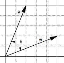
Let’s see what happens with two vectors, and , having an angle between (Figure 15).
On the one hand, adding them creates a new vector and the angle between   and is smaller than (Figure 16).

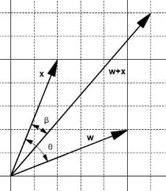
Figure 16: The addition creates a smaller angle

On the other hand, subtracting them creates a new vector , and the angle between and is bigger than (Figure 17).

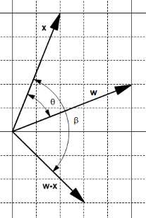
Figure 17: The subtraction creates a bigger angle

We can use these two observations to adjust the angle:

• If the predicted label is 1, the angle is smaller than . We want to increase the angle, so we set  .
• If the predicted label is -1, the angle is bigger than . We want to decrease the angle, so we set  .

As we are doing this only on misclassified examples, when the predicted label has a value, the expected label is the opposite. This means we can rewrite the previous statement:

• If the expected label is -1: We want to increase the angle, so we set  .
• If the expected label is +1: We want to decrease the angle, so we set  .

When translated into Python it gives us Code Listing 15, and we can see that it is strictly equivalent to Code Listing 16, which is the update rule.

Code Listing 15

Code Listing 16

We can verify that the update rule works as we expect by checking the value of the hypothesis before and after applying it (Code Listing 17).

Code Listing 17

Note that the update rule does not necessarily change the sign of the hypothesis for the example the first time. Sometimes it is necessary to apply the update rule several times before it happens as shown in Code Listing 18. This is not a problem, as we are looping across misclassified examples, so we will continue to use the update rule until the example is correctly classified. What matters here is that each time we use the update rule, we change the value of the angle in the right direction (increasing it or decreasing it).

Code Listing 18

Also note that sometimes updating the value of for a particular example changes the hyperplane in such a way that another example previously correctly classified becomes misclassified. So, the hypothesis might become worse at classifying after being updated. This is illustrated in Figure 18, which shows us the number of classified examples at each iteration step. One way to avoid this problem is to keep a record of the value of before making the update and use the updated only if it reduces the number of misclassified examples. This modification of the PLA is known as the Pocket algorithm (because we keep in our pocket).

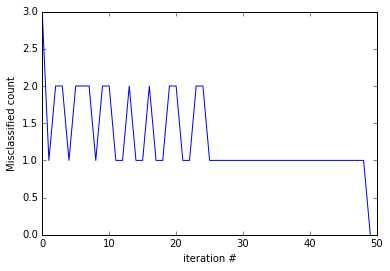
Figure 18: The PLA update rule oscillates

Convergence of the algorithm

We said that we keep updating the vector with the update rule until there is no misclassified point. But how can we be so sure that will ever happen? Luckily for us, mathematicians have studied this problem, and we can be very sure because the Perceptron convergence theorem guarantees that if the two sets P and N (of positive and negative examples respectively) are linearly separable, the vector is updated only a finite number of times, which was first proved by Novikoff in 1963 (Rojas, 1996).

Understanding the limitations of the PLA

One thing to understand about the PLA algorithm is that because weights are randomly initialized and misclassified examples are randomly chosen, it is possible the algorithm will return a different hyperplane each time we run it. Figure 19 shows the result of running the PLA on the same dataset four times. As you can see, the PLA finds four different hyperplanes.

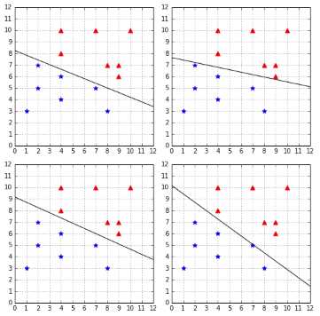
Figure 19: The PLA finds a different hyperplane each time

At first, this might not seem like a problem. After all, the four hyperplanes perfectly classify the data, so they might be equally good, right? However, when using a machine learning algorithm such as the PLA, our goal is not to find a way to classify perfectly the data we have right now. Our goal is to find a way to correctly classify new data we will receive in the future.

Let us introduce some terminology to be clear about this. To train a model, we pick a sample of existing data and call it the training set. We train the model, and it comes up with a hypothesis (a hyperplane in our case). We can measure how well the hypothesis performs on the training set: we call this the in-sample error (also called training error). Once we are satisfied with the hypothesis, we decide to use it on unseen data (the test set) to see if it indeed learned something. We measure how well the hypothesis performs on the test set, and we call this the out-of-sample error (also called the generalization error).

Our goal is to have the smallest out-of-sample error.

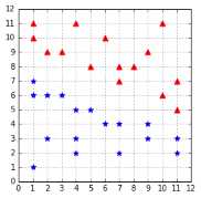
In the case of the PLA, all hypotheses in Figure 19 perfectly classify the data: their in-sample error is zero. But we are really concerned about their out-of-sample error. We can use a test set such as the one in Figure 20 to check their out-of-sample errors.

Figure 20: A test dataset

As you can see in Figure 21, the two hypotheses on the right, despite perfectly classifying the training dataset, are making errors with the test dataset.

Now we better understand why it is problematic. When using the Perceptron with a linearly separable dataset, we have the guarantee of finding a hypothesis with zero in-sample error, but we have no guarantee about how well it will generalize to unseen data (if an algorithm generalizes well, its out-of-sample error will be close to its in-sample error). How can we choose a hyperplane that generalizes well? As we will see in the next chapter, this is one of the goals of SVMs.

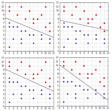
Figure 21: Not all hypotheses have perfect out-of-sample error

Summary

In this chapter, we have learned what a Perceptron is. We then saw in detail how the Perceptron Learning Algorithm works and what the motivation behind the update rule is. After learning that the PLA is guaranteed to converge, we saw that not all hypotheses are equal, and that some of them will generalize better than others. Eventually, we saw that the Perceptron is unable to select which hypothesis will have the smallest out-of-sample error and instead just picks one hypothesis having the lowest in-sample error at random.