Support Vector Machines Succinctly^®
by Alexandre Kowalczyk

CHAPTER 5

Solving the Optimization Problem

Lagrange multipliers

The Italian-French mathematician Giuseppe Lodovico Lagrangia, also known as Joseph-Louis Lagrange, invented a strategy for finding the local maxima and minima of a function subject to equality constraint. It is called the method of Lagrange multipliers.

The method of Lagrange multipliers

Lagrange noticed that when we try to solve an optimization problem of the form:

$%FontSize=11 %TeXFontSize=11 \documentclass{article} \pagestyle{empty} \begin{document} \begin{equation*} \begin{aligned} & \underset{\mathbf{x}}{\text{minimize}} & & f(\mathbf{x}) \\ & \text{subject to} & & g(\mathbf{x})=0 \end{aligned} \end{equation*} \end{document}$

the minimum of $%FontSize=11 %TeXFontSize=11 \documentclass{article} \pagestyle{empty} \begin{document} \[ f \] \end{document}$ is found when its gradient point in the same direction as the gradient of $%FontSize=11 %TeXFontSize=11 \documentclass{article} \pagestyle{empty} \begin{document} \[ g \] \end{document}$ .
In other words, when:

$%FontSize=11 %TeXFontSize=11 \documentclass{article} \pagestyle{empty} \begin{document} \[ \nabla f(\mathbf x) = \alpha \nabla g(\mathbf x) \] \end{document}$

So if we want to find the minimum of $%FontSize=11 %TeXFontSize=11 \documentclass{article} \pagestyle{empty} \begin{document} \[ f \] \end{document}$ under the constraint $%FontSize=11 %TeXFontSize=11 \documentclass{article} \pagestyle{empty} \begin{document} \[ g \] \end{document}$ , we just need to solve for:

$%FontSize=11 %TeXFontSize=11 \documentclass{article} \pagestyle{empty} \begin{document} \[ \nabla f(\mathbf x)-\alpha \nabla g(\mathbf x)=0 \] \end{document}$

Here, the constant $%FontSize=11 %TeXFontSize=11 \documentclass{article} \pagestyle{empty} \begin{document} \[ \alpha \] \end{document}$ is called a Lagrange multiplier.

To simplify the method, we observe that if we define a function $%FontSize=11 %TeXFontSize=11 \documentclass{article} \pagestyle{empty} \begin{document} \[ \mathcal{L}(\mathbf x,\alpha) = f(\mathbf x)-\alpha g(\mathbf x) \] \end{document}$ , then its gradient is $%FontSize=11 %TeXFontSize=11 \documentclass{article} \pagestyle{empty} \begin{document} \[ \nabla\mathcal{L}(\mathbf{x}, \alpha)= \nabla f(\mathbf x)-\alpha \nabla g(\mathbf x) \] \end{document}$ . As a result, solving for $%FontSize=11 %TeXFontSize=11 \documentclass{article} \pagestyle{empty} \begin{document} \[ \nabla\mathcal{L}(\mathbf{x}, \alpha)=0 \] \end{document}$ allows us to find the minimum.

The Lagrange multiplier method can be summarized by these three steps:

Construct the Lagrangian function $%FontSize=11 %TeXFontSize=11 \documentclass{article} \pagestyle{empty} \begin{document} \[ \mathcal{L} \] \end{document}$ by introducing one multiplier per constraint
Get the gradient $%FontSize=11 %TeXFontSize=11 \documentclass{article} \pagestyle{empty} \begin{document} \[ \nabla\mathcal{L} \] \end{document}$ of the Lagrangian
Solve for $%FontSize=11 %TeXFontSize=11 \documentclass{article} \pagestyle{empty} \begin{document} \[ \nabla\mathcal{L}(\mathbf{x}, \alpha)=0 \] \end{document}$

The SVM Lagrangian problem

We saw in the last chapter that the SVM optimization problem is:

$%FontSize=11 %TeXFontSize=11 \documentclass{article} \pagestyle{empty} \begin{document} \begin{equation*} \begin{aligned} & \underset{\mathbf{w},b}{\text{minimize}} & & \frac{1}{2}\|\mathbf{w}\|^2 \\ & \text{subject to} & & y_i(\mathbf{w}\cdot\mathbf{x}_i+b)-1 \geq 0 , \; i = 1, \ldots, m \\ \end{aligned} \end{equation*} \end{document}$

Let us return to this problem. We have one objective function to minimize:

$%FontSize=11 %TeXFontSize=11 \documentclass{article} \pagestyle{empty} \begin{document} $$f(\mathbf{w})=\frac{1}{2}\|\mathbf{w}\|^2$$\end{document}$

and $%FontSize=11 %TeXFontSize=11 \documentclass{article} \pagestyle{empty} \begin{document} \[ m \] \end{document}$ constraint functions:

$%FontSize=11 %TeXFontSize=11 \documentclass{article} \pagestyle{empty} \begin{document} $$g_i(\mathbf{w},b)= y_i(\mathbf{w}\cdot\mathbf{x}_i+b)-1, \; i = 1, \ldots, m $$\end{document}$

We introduce the Lagrangian function:

$%FontSize=11 %TeXFontSize=11 \documentclass{article} \pagestyle{empty} \begin{document} $$\mathcal{L}(\mathbf{w},b,\alpha)=f(\mathbf{w})- \sum\limits_{i=1}^m \alpha_i g_i(\mathbf{w},b)$$\end{document}$

$%FontSize=11 %TeXFontSize=11 \documentclass{article} \pagestyle{empty} \begin{document} $$ \mathcal{L}(\mathbf{w},b,\alpha)= \frac{1}{2}\|\mathbf{w}\|^2- \sum\limits_{i=1}^m \alpha_i\Big[ y_i(\mathbf{w}\cdot\mathbf{x}_i+b)-1\Big] $$ \end{document}$

Note that we introduced one Lagrange multiplier $%FontSize=11 %TeXFontSize=11 \documentclass{article} \pagestyle{empty} \begin{document} \[ \alpha_i \] \end{document}$ for each constraint function.

We could try to solve for , but the problem can only be solved analytically when the number of examples is small (Tyson Smith, 2004). So we will once again rewrite the problem using the duality principle.

To get the solution of the primal problem, we need to solve the following Lagrangian problem:

$%FontSize=11 %TeXFontSize=11 \documentclass{article} \pagestyle{empty} \begin{document} \begin{equation*} \begin{aligned} & \underset{\mathbf{w},b}{\text{min}}\quad\underset{\alpha}{\text{max}} & & \mathcal{L}(\mathbf{w},b,\alpha) \\ & \text{subject to} & & \alpha_i \geq 0 , \; \ i = 1, \ldots, m \\ \end{aligned} \end{equation*}\end{document}$

What is interesting here is that we need to minimize with respect to $%FontSize=11 %TeXFontSize=11 \documentclass{article} \pagestyle{empty} \begin{document} \[ \mathbf w \] \end{document}$ and $%FontSize=11 %TeXFontSize=11 \documentclass{article} \pagestyle{empty} \begin{document} \[ b \] \end{document}$ , and to maximize with respect to $%FontSize=11 %TeXFontSize=11 \documentclass{article} \pagestyle{empty} \begin{document} \[ \alpha \] \end{document}$ at the same time.

Tip: You may have noticed that the method of Lagrange multipliers is used for solving problems with equality constraints, and here we are using them with inequality constraints. This is because the method still works for inequality constraints, provided some additional conditions (the KKT conditions) are met. We will talk about these conditions later.

The Wolfe dual problem

The Lagrangian problem has $%FontSize=11 %TeXFontSize=11 \documentclass{article} \pagestyle{empty} \begin{document} \[ m \] \end{document}$ inequality constraints (where $%FontSize=11 %TeXFontSize=11 \documentclass{article} \pagestyle{empty} \begin{document} \[ m \] \end{document}$ is the number of training examples) and is typically solved using its dual form. The duality principle tells us that an optimization problem can be viewed from two perspectives. The first one is the primal problem, a minimization problem in our case, and the other one is the dual problem, which will be a maximization problem. What is interesting is that the maximum of the dual problem will always be less than or equal to the minimum of the primal problem (we say it provides a lower bound to the solution of the primal problem).

In our case, we are trying to solve a convex optimization problem, and Slater’s condition holds for affine constraints (Gretton, 2016), so Slater’s theorem tells us that strong duality holds. This means that the maximum of the dual problem is equal to the minimum of the primal problem. Solving the dual is the same thing as solving the primal, except it is easier.

Recall that the Lagrangian function is:

$%FontSize=11 %TeXFontSize=11 \documentclass{article} \pagestyle{empty} \begin{document} \begin{equation*} \begin{split} \mathcal{L}(\mathbf{w},b,\alpha) & = \frac{1}{2}\|\mathbf{w}\|^2- \sum\limits_{i=1}^m \alpha_i\big[y_i(\mathbf{w}\cdot\mathbf{x}_i+b)-1\big] \\ & = \frac{1}{2}\mathbf{w}\cdot\mathbf{w}- \sum\limits_{i=1}^m \alpha_i\big[y_i(\mathbf{w}\cdot\mathbf{x}_i+b)-1\big] \end{split} \end{equation*} \end{document}$

The Lagrangian primal problem is:

$%FontSize=11 %TeXFontSize=11 \documentclass{article} \pagestyle{empty} \begin{document} \begin{equation*} \begin{aligned} & \underset{\mathbf{w},b}{\text{min}}\quad\underset{\alpha}{\text{max}} & & \mathcal{L}(\mathbf{w},b,\alpha) \\ & \text{subject to} & & \alpha_i \geq 0 , \; \ i = 1, \ldots, m \\ \end{aligned} \end{equation*}\end{document}$

Solving the minimization problem involves taking the partial derivatives of $%FontSize=11 %TeXFontSize=11 \documentclass{article} \pagestyle{empty} \begin{document} \[ \mathcal{L} \] \end{document}$ with respect to $%FontSize=11 %TeXFontSize=11 \documentclass{article} \pagestyle{empty} \begin{document} \[ \mathbf w \] \end{document}$ and $%FontSize=11 %TeXFontSize=11 \documentclass{article} \pagestyle{empty} \begin{document} \[ b \] \end{document}$ .

$%FontSize=11 %TeXFontSize=11 \documentclass{article} \pagestyle{empty} \begin{document} \[ \nabla_\mathbf{w}\mathcal{L}= \mathbf{w}-\sum\limits_{i=1}^m \alpha_i y_i \mathbf{x}_i = \mathbf{0} \] \end{document}$

$%FontSize=11 %TeXFontSize=11 \documentclass{article} \pagestyle{empty} \begin{document} \[ \frac{\partial \mathcal{L}}{\partial b}=-\sum\limits_{i=1}^m \alpha_i y_i=0 \] \end{document}$

From the first equation, we find that:

$%FontSize=11 %TeXFontSize=11 \documentclass{article} \pagestyle{empty} \begin{document} \[ \mathbf{w}=\sum\limits_{i=1}^m \alpha_i y_i \mathbf{x}_i \] \end{document}$

Let us substitute $%FontSize=11 %TeXFontSize=11 \documentclass{article} \pagestyle{empty} \begin{document} \[ \mathbf{w} \] \end{document}$ by this value into $%FontSize=11 %TeXFontSize=11 \documentclass{article} \pagestyle{empty} \begin{document} \[ \mathcal{L} \] \end{document}$ :

$%FontSize=11 %TeXFontSize=11 \documentclass{article} \pagestyle{empty} \begin{document} \begin{equation*} \begin{split} W(\alpha,b) & = \frac{1}{2}\bigg(\sum\limits_{i=1}^m \alpha_i y_i \mathbf{x}_i\bigg)\cdot\bigg(\sum\limits_{j=1}^m \alpha_j y_j \mathbf{x}_j\bigg)- \sum\limits_{i=1}^m \alpha_i\bigg[y_i\bigg((\sum\limits_{j=1}^m \alpha_j y_j \mathbf{x}_j)\cdot\mathbf{x}_i+b\bigg)-1\bigg] \\ & = \frac{1}{2}\sum\limits_{i=1}^m \sum\limits_{j=1}^m \alpha_i\alpha_j y_i y_j \mathbf{x}_i\cdot \mathbf{x}_j- \sum\limits_{i=1}^m \alpha_i y_i\bigg((\sum\limits_{j=1}^m \alpha_j y_j \mathbf{x}_j)\cdot\mathbf{x}_i+b\bigg)+\sum\limits_{i=1}^m \alpha_i \\ & = \frac{1}{2}\sum\limits_{i=1}^m \sum\limits_{j=1}^m \alpha_i\alpha_j y_i y_j \mathbf{x}_i\cdot \mathbf{x}_j- \sum\limits_{i=1}^m \sum\limits_{j=1}^m \alpha_i \alpha_j y_i y_j \mathbf{x}_i\cdot\mathbf{x}_j -b\sum\limits_{i=1}^m \alpha_i y_i +\sum\limits_{i=1}^m \alpha_i \\ & = \sum\limits_{i=1}^m \alpha_i -\frac{1}{2}\sum\limits_{i=1}^m \sum\limits_{j=1}^m \alpha_i\alpha_j y_i y_j \mathbf{x}_i\cdot \mathbf{x}_j -b\sum\limits_{i=1}^m \alpha_i y_i \end{split} \end{equation*} \end{document}$

So we successfully removed $%FontSize=11 %TeXFontSize=11 \documentclass{article} \pagestyle{empty} \begin{document} \[ \mathbf{w} \] \end{document}$ , but $%FontSize=11 %TeXFontSize=11 \documentclass{article} \pagestyle{empty} \begin{document} \[ b \] \end{document}$ is still used in the last term of the function:

$%FontSize=11 %TeXFontSize=11 \documentclass{article} \pagestyle{empty} \begin{document} \begin{equation*} W(\alpha,b) = \sum\limits_{i=1}^m \alpha_i -\frac{1}{2}\sum\limits_{i=1}^m \sum\limits_{j=1}^m \alpha_i\alpha_j y_i y_j \mathbf{x}_i\cdot \mathbf{x}_j -b\sum\limits_{i=1}^m \alpha_i y_i \end{equation*} \end{document}$

We note that $%FontSize=11 %TeXFontSize=11 \documentclass{article} \pagestyle{empty} \begin{document} \[ \frac{\partial \mathcal{L}}{\partial b}=0 \] \end{document}$ implies that $%FontSize=11 %TeXFontSize=11 \documentclass{article} \pagestyle{empty} \begin{document} $\sum\limits_{i=1}^m \alpha_i y_i=0$ \end{document}$ . As a result, the last term is equal to zero, and we can write:

$%FontSize=11 %TeXFontSize=11 \documentclass{article} \pagestyle{empty} \begin{document} \begin{equation*} W(\alpha) = \sum\limits_{i=1}^m \alpha_i -\frac{1}{2}\sum\limits_{i=1}^m \sum\limits_{j=1}^m \alpha_i\alpha_j y_i y_j \mathbf{x}_i\cdot \mathbf{x}_j \end{equation*} \end{document}$

This is the Wolfe dual Lagrangian function.

The optimization problem is now called the Wolfe dual problem:

$%FontSize=11 %TeXFontSize=11 \documentclass{article} \pagestyle{empty} \begin{document} \begin{equation*} \begin{aligned} & \underset{\alpha}{\text{maximize}} & & \sum\limits_{i=1}^m \alpha_i -\frac{1}{2}\sum\limits_{i=1}^m \sum\limits_{j=1}^m \alpha_i\alpha_j y_i y_j \mathbf{x}_i\cdot \mathbf{x}_j \\ & \text{subject to} & & \alpha_i \geq 0 , \; \text{for any}\ i = 1, \ldots, m \\ & & & \sum\limits_{i=1}^m \alpha_i y_i=0 \\ \end{aligned} \end{equation*}\end{document}$

Traditionally the Wolfe dual Lagrangian problem is constrained by the gradients being equal to zero. In theory, we should add the constraints $%FontSize=11 %TeXFontSize=11 \documentclass{article} \pagestyle{empty} \begin{document} $ \nabla_\mathbf{w}\mathcal{L}=0 $ \end{document}$ and $%FontSize=11 %TeXFontSize=11 \documentclass{article} \pagestyle{empty} \begin{document} $ \frac{\partial \mathcal{L}}{\partial b}=0 $ \end{document}$ . However, we only added the latter. Indeed, we added $%FontSize=11 %TeXFontSize=11 \documentclass{article} \pagestyle{empty} \begin{document} $\sum\limits_{i=1}^m \alpha_i y_i=0$ \end{document}$ because it is necessary for removing $%FontSize=11 %TeXFontSize=11 \documentclass{article} \pagestyle{empty} \begin{document} \[ b \] \end{document}$ from the function. However, we can solve the problem without the constraint $%FontSize=11 %TeXFontSize=11 \documentclass{article} \pagestyle{empty} \begin{document} $\mathbf{w}=\sum\limits_{i=1}^m \alpha_i y_i \mathbf{x}_i$ \end{document}$ .

The main advantage of the Wolfe dual problem over the Lagrangian problem is that the objective function $%FontSize=11 %TeXFontSize=11 \documentclass{article} \pagestyle{empty} \begin{document} \[ W \] \end{document}$ now depends only on the Lagrange multipliers. Moreover, this formulation will help us solve the problem in Python in the next section and will be very helpful when we define kernels later.

Karush-Kuhn-Tucker conditions

Because we are dealing with inequality constraints, there is an additional requirement: the solution must also satisfy the Karush-Kuhn-Tucker (KKT) conditions.

The KKT conditions are first-order necessary conditions for a solution of an optimization problem to be optimal. Moreover, the problem should satisfy some regularity conditions. Luckily for us, one of the regularity conditions is Slater’s condition, and we just saw that it holds for SVMs. Because the primal problem we are trying to solve is a convex problem, the KKT conditions are also sufficient for the point to be primal and dual optimal, and there is zero duality gap.

To sum up, if a solution satisfies the KKT conditions, we are guaranteed that it is the optimal solution.

The Karush-Kuhn-Tucker conditions are:

Stationarity condition:

$%FontSize=11 %TeXFontSize=11 \documentclass{article} \pagestyle{empty} \begin{document} \[ \frac{\partial \mathcal{L}}{\partial b}=-\sum\limits_{i=1}^m \alpha_i y_i=0 \] \end{document}$

Primal feasibility condition:

$%FontSize=11 %TeXFontSize=11 \documentclass{article} \pagestyle{empty} \begin{document} \[ y_i(\mathbf{w}\cdot\mathbf{x}_i+b)-1 \geq 0 \quad \quad \text{for all}\ i = 1,\dots,m \] \end{document}$

Dual feasibility condition:

$%FontSize=11 %TeXFontSize=11 \documentclass{article} \pagestyle{empty} \begin{document} \[ \alpha_i \geq 0 \quad \quad \text{for all}\ i = 1,\dots,m \] \end{document}$

Complementary slackness condition:

$%FontSize=11 %TeXFontSize=11 \documentclass{article} \pagestyle{empty} \begin{document} \[ \alpha_i\big[y_i(\mathbf{w}\cdot\mathbf{x}_i+b)-1\big] = 0 \quad \quad \text{for all}\ i = 1,\dots,m \] \end{document}$

Note: “[...]Solving the SVM problem is equivalent to finding a solution to the KKT conditions.” (Burges, 1988)

Note that we already saw most of these conditions before. Let us examine them one by one.

Stationarity condition

The stationarity condition tells us that the selected point must be a stationary point. It is a point where the function stops increasing or decreasing. When there is no constraint, the stationarity condition is just the point where the gradient of the objective function is zero. When we have constraints, we use the gradient of the Lagrangian.

Primal feasibility condition

Looking at this condition, you should recognize the constraints of the primal problem. It makes sense that they must be enforced to find the minimum of the function under constraints.

Dual feasibility condition

Similarly, this condition represents the constraints that must be respected for the dual problem.

Complementary slackness condition

From the complementary slackness condition, we see that either $%FontSize=11 %TeXFontSize=11 \documentclass{article} \pagestyle{empty} \begin{document} \[ \alpha_i = 0 \] \end{document}$ or $%FontSize=11 %TeXFontSize=11 \documentclass{article} \pagestyle{empty} \begin{document} \[ y_i(\mathbf{w}\cdot\mathbf{x}_i+b)-1 = 0 \] \end{document}$ .

Support vectors are examples having a positive Lagrange multiplier. They are the ones for which the constraint $%FontSize=11 %TeXFontSize=11 \documentclass{article} \pagestyle{empty} \begin{document} \[ y_i(\mathbf{w}\cdot\mathbf{x}_i+b)-1 \geq 0 \] \end{document}$ is active. (We say the constraint is active when $%FontSize=11 %TeXFontSize=11 \documentclass{article} \pagestyle{empty} \begin{document} \[ y_i(\mathbf{w}\cdot\mathbf{x}_i+b)-1 = 0 \] \end{document}$ ).

Tip: From the complementary slackness condition, we see that support vectors are examples that have a positive Lagrange multiplier.

What to do once we have the multipliers?

When we solve the Wolfe dual problem, we get a vector $%FontSize=11 %TeXFontSize=11 \documentclass{article} \pagestyle{empty} \begin{document} \[ \alpha \] \end{document}$ containing all Lagrange multipliers. However, when we first stated the primal problem, our goal was to find $%FontSize=11 %TeXFontSize=11 \documentclass{article} \pagestyle{empty} \begin{document} $ \mathbf{w} $ \end{document}$ and $%FontSize=11 %TeXFontSize=11 \documentclass{article} \pagestyle{empty} \begin{document} $ b $ \end{document}$ . Let us see how we can retrieve these values from the Lagrange multipliers.

Compute w

Computing $%FontSize=11 %TeXFontSize=11 \documentclass{article} \pagestyle{empty} \begin{document} $ \mathbf{w} $ \end{document}$ is pretty simple since we derived the formula: $%FontSize=11 %TeXFontSize=11 \documentclass{article} \pagestyle{empty} \begin{document} $\mathbf{w}=\sum\limits_{i=1}^m \alpha_i y_i \mathbf{x}_i$ \end{document}$ from the gradient $%FontSize=11 %TeXFontSize=11 \documentclass{article} \pagestyle{empty} \begin{document} $ \nabla_\mathbf{w}\mathcal{L} $ \end{document}$ .

Compute b

Once we have $%FontSize=11 %TeXFontSize=11 \documentclass{article} \pagestyle{empty} \begin{document} $ \mathbf{w} $ \end{document}$ , we can use one of the constraints of the primal problem to compute $%FontSize=11 %TeXFontSize=11 \documentclass{article} \pagestyle{empty} \begin{document} $ b $ \end{document}$ :

$%FontSize=11 %TeXFontSize=11 \documentclass{article} \pagestyle{empty} \begin{document} \[ y_i(\mathbf{w}\cdot\mathbf{x}_i+b)-1\geq0 \] \end{document}$

Indeed, this constraint is still true because we transformed the original problem in such a way that the new formulations are equivalent. What it says is that the closest points to the hyperplane will have a functional margin of 1 (the value 1 is the value we chose when we decided how to scale $%FontSize=11 %TeXFontSize=11 \documentclass{article} \pagestyle{empty} \begin{document} $ \mathbf{w} $ \end{document}$ ):

$%FontSize=11 %TeXFontSize=11 \documentclass{article} \pagestyle{empty} \begin{document} \[ y_i(\mathbf{w}\cdot\mathbf{x}_i+b)=1 \] \end{document}$

From there, as we know all other variables, it is easy to come up with the value of $%FontSize=11 %TeXFontSize=11 \documentclass{article} \pagestyle{empty} \begin{document} $ b $ \end{document}$ . We multiply both sides of the equation by $%FontSize=11 %TeXFontSize=11 \documentclass{article} \pagestyle{empty} \begin{document} $y_i$ \end{document}$ , and because $%FontSize=11 %TeXFontSize=11 \documentclass{article} \pagestyle{empty} \begin{document} $ y_i^2=1 $ \end{document}$ , it gives us:

$%FontSize=11 %TeXFontSize=11 \documentclass{article} \pagestyle{empty} \begin{document} \[ \mathbf{w}\cdot\mathbf{x}_i+b=y_i \] \end{document}$

$%FontSize=11 %TeXFontSize=11 \documentclass{article} \pagestyle{empty} \begin{document} \[ b=y_i-\mathbf{w}\cdot\mathbf{x}_i \] \end{document}$

However, as indicated in Pattern Recognition and Machine Learning (Bishop, 2006), instead of taking a random support vector $%FontSize=11 %TeXFontSize=11 \documentclass{article} \pagestyle{empty} \begin{document} $ \mathbf{x}_i $ \end{document}$ , taking the average provides us with a numerically more stable solution:

$%FontSize=11 %TeXFontSize=11 \documentclass{article} \pagestyle{empty} \begin{document} \[ b=\frac{1}{S}\sum\limits_{i=1}^S (y_i-\mathbf{w}\cdot\mathbf{x}_i) \] \end{document}$

where $%FontSize=11 %TeXFontSize=11 \documentclass{article} \pagestyle{empty} \begin{document} $ S $ \end{document}$ is the number of support vectors.

Other authors, such as (Cristianini & Shawe-Taylor, 2000) and (Ng), use another formula:

$%FontSize=11 %TeXFontSize=11 \documentclass{article} \pagestyle{empty} \begin{document} \[ b=-\frac{max_{y_i=-1}(\mathbf{w}\cdot\mathbf{x}_i)+min_{y_i=1}(\mathbf{w}\cdot\mathbf{x}_i)}{2} \] \end{document}$

They basically take the average of the nearest positive support vector and the nearest negative support vector. This latest formula is the one originally used by Statistical Learning Theory (Vapnik V. N., 1998) when defining the optimal hyperplane.

Hypothesis function

The SVMs use the same hypothesis function as the Perceptron. The class of an example $%FontSize=11 %TeXFontSize=11 \documentclass{article} \pagestyle{empty} \begin{document} \[ \mathbf{x}_i \] \end{document}$ is given by:

$%FontSize=11 %TeXFontSize=11 \documentclass{article} \pagestyle{empty} \begin{document} \[ h(\mathbf{x}_i)=\text{sign}(\mathbf{w}\cdot\mathbf{x}_i+b) \] \end{document}$

When using the dual formulation, it is computed using only the support vectors:

$%FontSize=11 %TeXFontSize=11 ontSize=11 %TeXFontSize=11 \documentclass{article} \pagestyle{empty} \begin{document} \[ h(\mathbf{x}_i)=\text{sign}\Bigg(\sum\limits_{j=1}^S \alpha_j y_j(\mathbf{x}_j\cdot\mathbf{x}_i)+b\Bigg) \] \end{document}$

Solving SVMs with a QP solver

A QP solver is a program used to solve quadratic programming problems. In the following example, we will use the Python package called CVXOPT.

This package provides a method that is able to solve quadratic problems of the form:

$%FontSize=11 %TeXFontSize=11 \documentclass{article} \pagestyle{empty} \begin{document} \begin{equation*} \begin{aligned} & \underset{x}{\text{minimize}} & & \frac{1}{2} x^TPx + q^T x \\ & \text{subject to} & & Gx \preceq h \\ & & & Ax = b \\ \end{aligned} \end{equation*}\end{document}$

It does not look like our optimization problem, so we will need to rewrite it so that we can solve it with this package.

First, we note that in the case of the Wolfe dual optimization problem, what we are trying to minimize is $%FontSize=11 %TeXFontSize=11 \documentclass{article} \pagestyle{empty} \begin{document} \[ \alpha \] \end{document}$ , so we can rewrite the quadratic problem with $%FontSize=11 %TeXFontSize=11 \documentclass{article} \pagestyle{empty} \begin{document} \[ \alpha \] \end{document}$ instead of $%FontSize=11 %TeXFontSize=11 \documentclass{article} \pagestyle{empty} \begin{document} \[ x \] \end{document}$ to better see how the two problems relate:

$%FontSize=11 %TeXFontSize=11 \documentclass{article} \pagestyle{empty} \begin{document} \begin{equation*} \begin{aligned} & \underset{x}{\text{minimize}} & & \frac{1}{2} \alpha^TP\alpha + q^T \alpha \\ & \text{subject to} & & G\alpha \preceq h \\ & & & A\alpha = b \\ \end{aligned} \end{equation*}\end{document}$

Here the $%FontSize=11 %TeXFontSize=11 \documentclass{article} \pagestyle{empty} \begin{document} $\preceq$ \end{document}$ symbol represents component-wise vector inequalities. It means that each row of the matrix $%FontSize=11 %TeXFontSize=11 \documentclass{article} \pagestyle{empty} \begin{document} $G\lambda$ \end{document}$ represents an inequality that must be satisfied.

We will change the Wolfe dual problem. First, we transform the maximization problem:

$%FontSize=11 %TeXFontSize=11 \documentclass{article} \pagestyle{empty} \begin{document} \begin{equation*} \begin{aligned} & \underset{\alpha}{\text{maximize}} & & -\frac{1}{2}\sum\limits_{i=1}^m \sum\limits_{j=1}^m \alpha_i\alpha_j y_i y_j \mathbf{x}_i\cdot \mathbf{x}_j + \sum\limits_{i=1}^m \alpha_i \\ & \text{subject to} & & \alpha_i \geq 0 , \; \text{for any}\ i = 1, \ldots, m \\ & & & \sum\limits_{i=1}^m \alpha_i y_i=0 \\ \end{aligned} \end{equation*}\end{document}$

into a minimization problem by multiplying by -1.

$%FontSize=11 %TeXFontSize=11 \documentclass{article} \pagestyle{empty} \begin{document} \begin{equation*} \begin{aligned} & \underset{\alpha}{\text{minimize}} & & \frac{1}{2}\sum\limits_{i=1}^m \sum\limits_{j=1}^m \alpha_i\alpha_j y_i y_j \mathbf{x}_i\cdot \mathbf{x}_j-\sum\limits_{i=1}^m \alpha_i \\ & \text{subject to} & & -\alpha_i \leq 0 , \; \text{for any}\ i = 1, \ldots, m \\ & & & \sum\limits_{i=1}^m \alpha_i y_i=0 \\ \end{aligned} \end{equation*} \end{document}$

Then we introduce vectors $%FontSize=11 %TeXFontSize=11 \documentclass{article} \pagestyle{empty} \begin{document} $\alpha = (\alpha_1, \dots, \alpha_m)^T$\end{document}$ and $%FontSize=11 %TeXFontSize=11 \documentclass{article} \pagestyle{empty} \begin{document} $\mathbf{y} = (y_1, \cdots,y_m)^T$ \end{document}$ and the Gram matrix $%FontSize=11 %TeXFontSize=11 \documentclass{article} \pagestyle{empty} \begin{document} $K$ \end{document}$ of all possible dot products of vectors $%FontSize=11 %TeXFontSize=11 \documentclass{article} \pagestyle{empty} \begin{document} $\mathbf{x}_i$\end{document}$ :

$%FontSize=11 %TeXFontSize=11 \documentclass{article} \pagestyle{empty} \begin{document} $${\displaystyle K(\mathbf{x}_{1},\dots ,\mathbf{x}_{m})={\begin{pmatrix}\mathbf{x}_{1}\cdot \mathbf{x}_{1} &\mathbf{x}_{1}\cdot\mathbf{x}_{2} &\dots & \mathbf{x}_{1}\cdot\mathbf{x}_{m} \\ \mathbf{x}_{2}\cdot\mathbf{x}_{1} & \mathbf{x}_{2}\cdot\mathbf{x}_{2} &\dots & \mathbf{x}_{2}\cdot\mathbf{x}_{m} \\\vdots &\vdots &\ddots &\vdots \\ \mathbf{x}_{m}\cdot\mathbf{x}_{1} & \mathbf{x}_{m}\cdot\mathbf{x}_{2} &\dots & \mathbf{x}_{m}\cdot\mathbf{x}_{m} \end{pmatrix}}}$$ \end{document}$

We use them to construct a vectorized version of the Wolfe dual problem where $%FontSize=11 %TeXFontSize=11 \documentclass{article} \pagestyle{empty} \begin{document} $\mathbf{y}\mathbf{y}^T$ \end{document}$ denotes the outer product of $%FontSize=11 %TeXFontSize=11 \documentclass{article} \pagestyle{empty} \begin{document} $\mathbf{y}$ \end{document}$ .

$%FontSize=11 %TeXFontSize=11 \documentclass{article} \pagestyle{empty} \begin{document} \begin{equation*} \begin{aligned} & \underset{\alpha}{\text{minimize}} & & \frac{1}{2} \alpha^T (\mathbf{y}\mathbf{y}^TK) \alpha - \alpha \\ & \text{subject to} & & -\alpha \preceq 0 , \; \\ & & & \mathbf{y}\cdot\alpha=0 \\ \end{aligned} \end{equation*}\end{document}$

We are now able to find out the value for each of the parameters $%FontSize=11 %TeXFontSize=11 \documentclass{article} \pagestyle{empty} \begin{document} \[ P \] \end{document}$ , $%FontSize=11 %TeXFontSize=11 \documentclass{article} \pagestyle{empty} \begin{document} \[ q \] \end{document}$ , $%FontSize=11 %TeXFontSize=11 \documentclass{article} \pagestyle{empty} \begin{document} \[ G \] \end{document}$ , $%FontSize=11 %TeXFontSize=11 \documentclass{article} \pagestyle{empty} \begin{document} \[ h \] \end{document}$ , $%FontSize=11 %TeXFontSize=11 \documentclass{article} \pagestyle{empty} \begin{document} \[ A \] \end{document}$ , and $%FontSize=11 %TeXFontSize=11 \documentclass{article} \pagestyle{empty} \begin{document} \[ b \] \end{document}$ required by the CVXOPT qp function. This is demonstrated in Code Listing 24.

Code Listing 24

# See Appendix A for more information about the dataset

from succinctly.datasets import get_dataset, linearly_separable as ls

import cvxopt.solvers

X, y = get_dataset(ls.get_training_examples)
m = X.shape[0]

# Gram matrix - The matrix of all possible inner products of X.
K = np.array([np.dot(X[i], X[j])
for j in range(m)
for i in range(m)]).reshape((m, m))

P = cvxopt.matrix(np.outer(y, y) * K)
q = cvxopt.matrix(-1 * np.ones(m))

# Equality constraints
A = cvxopt.matrix(y, (1, m))
b = cvxopt.matrix(0.0)

# Inequality constraints
G = cvxopt.matrix(np.diag(-1 * np.ones(m)))
h = cvxopt.matrix(np.zeros(m))

# Solve the problem
solution = cvxopt.solvers.qp(P, q, G, h, A, b)

# Lagrange multipliers
multipliers = np.ravel(solution['x'])

# Support vectors have positive multipliers.
has_positive_multiplier = multipliers > 1e-7
sv_multipliers = multipliers[has_positive_multiplier]

support_vectors = X[has_positive_multiplier]
support_vectors_y = y[has_positive_multiplier]

Code Listing 24 initializes all the required parameters and passes them to the qp function, which returns us a solution. The solution contains many elements, but we are only concerned about the x, which, in our case, corresponds to the Lagrange multipliers.

As we saw before, we can re-compute using all the Lagrange multipliers: $%FontSize=11 %TeXFontSize=11 \documentclass{article} \pagestyle{empty} \begin{document} $\mathbf{w}=\sum\limits_{i=1}^m \alpha_i y_i \mathbf{x}_i$ \end{document}$ . Code Listing 25 shows the code of the function that computes .

Code Listing 25

def compute_w(multipliers, X, y):
return np.sum(multipliers[i] * y[i] * X[i]
for i in range(len(y)))

Because Lagrange multipliers for non-support vectors are almost zero, we can also compute using only support vectors data and their multipliers, as illustrated in Code Listing 26.

Code Listing 26

w = compute_w(multipliers, X, y)
w_from_sv = compute_w(sv_multipliers, support_vectors, support_vectors_y)

print(w) # [0.44444446 1.11111114]
print(w_from_sv) # [0.44444453 1.11111128]

And we compute b using the average method:

Code Listing 27

def compute_b(w, X, y):
return np.sum([y[i] - np.dot(w, X[i])
for i in range(len(X))])/len(X)

Code Listing 28

b = compute_b(w, support_vectors, support_vectors_y) # -9.666668268506335

When we plot the result in Figure 32, we see that the hyperplane is the optimal hyperplane. Contrary to the Perceptron, the SVM will always return the same result.

The hyperplane found with CVXOPT

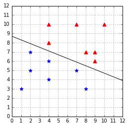
Figure 32: The hyperplane found with CVXOPT

This formulation of the SVM is called the hard margin SVM. It cannot work when the data is not linearly separable. There are several Support Vector Machines formulations. In the next chapter, we will consider another formulation called the soft margin SVM, which will be able to work when data is non-linearly separable because of outliers.

Summary

Minimizing the norm of $%FontSize=11 %TeXFontSize=11 \documentclass{article} \pagestyle{empty} \begin{document} \[ \mathbf{w} \] \end{document}$ is a convex optimization problem, which can be solved using the Lagrange multipliers method. When there are more than a few examples, we prefer using convex optimization packages, which will do all the hard work for us.

We saw that the original optimization problem can be rewritten using a Lagrangian function. Then, thanks to duality theory, we transformed the Lagrangian problem into the Wolfe dual problem. We eventually used the package CVXOPT to solve the Wolfe dual.

Build apps 2X faster

using Syncfusion Essential Studio^® suite

1800+ high-performance UI components.
Includes popular controls such as Grid, Chart, Scheduler, and more.
24x5 unlimited support by developers.

Get Your Free Trial Now