Support Vector Machines Succinctly^®
by Alexandre Kowalczyk

CHAPTER 6

Soft Margin SVM

Dealing with noisy data

The biggest issue with hard margin SVM is that it requires the data to be linearly separable. Real-life data is often noisy. Even when the data is linearly separable, a lot of things can happen before you feed it to your model. Maybe someone mistyped a value for an example, or maybe the probe of a sensor returned a crazy value. In the presence of an outlier (a data point that seems to be out of its group), there are two cases: the outlier can be closer to the other examples than most of the examples of its class, thus reducing the margin, or it can be among the other examples and break linear separability. Let us consider these two cases and see how the hard margin SVM deals with them.

Outlier reducing the margin

When the data is linearly separable, the hard margin classifier does not behave as we would like in the presence of outliers.

Let us now consider our dataset with the addition of an outlier data point at (5, 7), as shown in Figure 33.

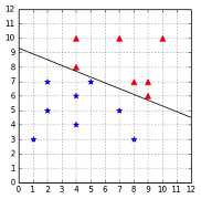
The dataset is still linearly separable with the outlier at (5, 7)

Figure 33: The dataset is still linearly separable with the outlier at (5, 7)

In this case, we can see that the margin is very narrow, and it seems that the outlier is the main reason for this change. Intuitively, we can see that this hyperplane might not be the best at separating the data, and that it will probably generalize poorly.

Outlier breaking linear separability

Even worse, when the outlier breaks the linear separability, as the point (7, 8) does in Figure 34, the classifier is incapable of finding a hyperplane. We are stuck because of a single data point.

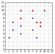
The outlier at (7, 8) breaks linear separability

Figure 34: The outlier at (7, 8) breaks linear separability

Soft margin to the rescue

Slack variables

In 1995, Vapnik and Cortes introduced a modified version of the original SVM that allows the classifier to make some mistakes. The goal is now not to make zero classification mistakes, but to make as few mistakes as possible.

To do so, they modified the constraints of the optimization problem by adding a variable $%FontSize=11 %TeXFontSize=11 \documentclass{article} \pagestyle{empty} \begin{document} $\zeta$ \end{document}$ (zeta). So the constraint:

$%FontSize=11 %TeXFontSize=11 \documentclass{article} \pagestyle{empty} \begin{document} $$y_i(\mathbf{w}\cdot\mathbf{x}_i+b)\geq 1$$ \end{document}$

becomes:

$%FontSize=11 %TeXFontSize=11 \documentclass{article} \pagestyle{empty} \begin{document} \[ y_i(\mathbf{w}\cdot\mathbf{x}_i+b)\geq 1 - \zeta_i \] \end{document}$

As a result, when minimizing the objective function, it is possible to satisfy the constraint even if the example does not meet the original constraint (that is, it is too close from the hyperplane, or it is not on the correct side of the hyperplane). This is illustrated in Code Listing 29.

Code Listing 29

import numpy as np

w = np.array([0.4, 1])
b = -10

x = np.array([6, 8])
y = -1

def constraint(w, b, x, y):
return y * (np.dot(w, x) + b)

def hard_constraint_is_satisfied(w, b, x, y):
    return constraint(w, b, x, y) >= 1

def soft_constraint_is_satisfied(w, b, x, y, zeta):
    return constraint(w, b, x, y) >= 1 - zeta

# While the constraint is not satisfied for the example (6,8).
print(hard_constraint_is_satisfied(w, b, x, y))               # False

# We can use zeta = 2 and satisfy the soft constraint.
print(soft_constraint_is_satisfied(w, b, x, y, zeta=2))       # True

The problem is that we could choose a huge value of $%FontSize=11 %TeXFontSize=11 \documentclass{article} \pagestyle{empty} \begin{document} $\zeta$ \end{document}$ for every example, and all the constraints will be satisfied.

Code Listing 30

# We can pick a huge zeta for every point
# to always satisfy the soft constraint.
print(soft_constraint_is_satisfied(w, b, x, y, zeta=10)) # True
print(soft_constraint_is_satisfied(w, b, x, y, zeta=1000)) # True

To avoid this, we need to modify the objective function to penalize the choice of a big $%FontSize=11 %TeXFontSize=11 \documentclass{article} \pagestyle{empty} \begin{document} $\zeta_i$ \end{document}$ :

$%FontSize=11 %TeXFontSize=11 \documentclass{article} \pagestyle{empty} \begin{document} \[ \begin{equation*} \begin{aligned} & \underset{\mathbf{w},b,\zeta}{\text{minimize}} && \frac{1}{2}\|\mathbf{w}\|^2 + \sum\limits_{i=1}^{m}\zeta_i \\ & \text{subject to} & & y_i(\mathbf{w}\cdot\mathbf{x}_i+b)\geq 1 - \zeta_i\quad \text{for any}\ i = 1, \ldots, m \\ \end{aligned} \end{equation*} \] \end{document}$

We take the sum of all individual $%FontSize=11 %TeXFontSize=11 \documentclass{article} \pagestyle{empty} \begin{document} $\zeta_i$ \end{document}$ and add it to the objective function. Adding such a penalty is called regularization. As a result, the solution will be the hyperplane that maximizes the margin while having the smallest error possible.

There is still a little problem. With this formulation, one can easily minimize the function by using negative values of $%FontSize=11 %TeXFontSize=11 \documentclass{article} \pagestyle{empty} \begin{document} $\zeta_i$ \end{document}$ . We add the constraint $%FontSize=11 %TeXFontSize=11 \documentclass{article} \pagestyle{empty} \begin{document} \[ \zeta_i \geq 0 \] \end{document}$ to prevent this. Moreover, we would like to keep some control over the soft margin. Maybe sometimes we want to use the hard margin—after all, that is why we add the parameter $%FontSize=11 %TeXFontSize=11 \documentclass{article} \pagestyle{empty} \begin{document} \[ C \] \end{document}$ , which will help us to determine how important the $%FontSize=11 %TeXFontSize=11 \documentclass{article} \pagestyle{empty} \begin{document} $\zeta$ \end{document}$ should be (more on that later).

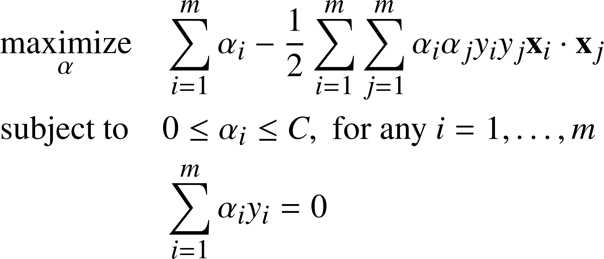
This leads us to the soft margin formulation:

$%FontSize=11 %TeXFontSize=11 \documentclass{article} \pagestyle{empty} \begin{document} $$ \begin{equation*} \begin{aligned} & \underset{\mathbf{w},b,\zeta}{\text{minimize}} && \frac{1}{2}\|\mathbf{w}\|^2 + C\sum\limits_{i=1}^{m}\zeta_i \\ & \text{subject to} & & y_i(\mathbf{w}\cdot\mathbf{x}_i+b)\geq 1 - \zeta_i\\ & & & \zeta_i \geq 0\quad\text{for any}\ i = 1, \ldots, m \\ \end{aligned} \end{equation*} $$ \end{document}$

As shown by (Vapnik V. N., 1998), using the same technique as for the separable case, we find that we need to maximize the same Wolfe dual as before, under a slightly different constraint:

Here the constraint $%FontSize=11 %TeXFontSize=11 \documentclass{article} \pagestyle{empty} \begin{document} \[ \alpha_i \geq 0 \] \end{document}$ has been changed to become $%FontSize=11 %TeXFontSize=11 \documentclass{article} \pagestyle{empty} \begin{document} \[ 0 \leq \alpha_i \leq C \] \end{document}$ . This constraint is often called the box constraint because the vector $%FontSize=11 %TeXFontSize=11 \documentclass{article} \pagestyle{empty} \begin{document} \[ \alpha \] \end{document}$ is constrained to lie inside the box with side length $%FontSize=11 %TeXFontSize=11 \documentclass{article} \pagestyle{empty} \begin{document} \[ C \] \end{document}$ in the positive orthant. Note that an orthant is the analog n-dimensional Euclidean space of a quadrant in the plane (Cristianini & Shawe-Taylor, 2000). We will visualize the box constraint in Figure 50 in the chapter about the SMO algorithm.

The optimization problem is also called 1-norm soft margin because we are minimizing the 1-norm of the slack vector $%FontSize=11 %TeXFontSize=11 \documentclass{article} \pagestyle{empty} \begin{document} \[ \mathbf{\zeta} \] \end{document}$ .

Understanding what C does

The parameter gives you control of how the SVM will handle errors. Let us now examine how changing its value will give different hyperplanes.

Figure 35 shows the linearly separable dataset we used throughout this book. On the left, we can see that setting $%FontSize=11 %TeXFontSize=11 \documentclass{article} \pagestyle{empty} \begin{document} \[ C \] \end{document}$ to $%FontSize=11 %TeXFontSize=11 \documentclass{article} \pagestyle{empty} \begin{document} \[ +\inf \] \end{document}$ gives us the same result as the hard margin classifier. However, if we choose a smaller value for $%FontSize=11 %TeXFontSize=11 \documentclass{article} \pagestyle{empty} \begin{document} \[ C \] \end{document}$ like we did in the center, we can see that the hyperplane is closer to some points than others. The hard margin constraint is violated for these examples. Setting $%FontSize=11 %TeXFontSize=11 \documentclass{article} \pagestyle{empty} \begin{document} \[ C=0.01 \] \end{document}$ increases this behavior as depicted on the right.

What happens if we choose a $%FontSize=11 %TeXFontSize=11 \documentclass{article} \pagestyle{empty} \begin{document} \[ C \] \end{document}$ very close to zero? Then there is basically no constraint anymore, and we end up with a hyperplane not classifying anything.

Effect of C=+Infinity, C=1, and C=0.01 on a linearly separable dataset

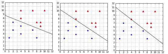
Figure 35: Effect of C=+Infinity, C=1, and C=0.01 on a linearly separable dataset

It seems that when the data is linearly separable, sticking with a big $%FontSize=11 %TeXFontSize=11 \documentclass{article} \pagestyle{empty} \begin{document} \[ C \] \end{document}$ is the best choice. But what if we have some noisy outlier? In this case, as we can see in Figure 36, using $%FontSize=11 %TeXFontSize=11 \documentclass{article} \pagestyle{empty} \begin{document} \[ C=+\infty \] \end{document}$ gives us a very narrow margin. However, when we use $%FontSize=11 %TeXFontSize=11 \documentclass{article} \pagestyle{empty} \begin{document} \[ C=1 \] \end{document}$ , we end up with a hyperplane very close to the one of the hard margin classifier without outlier. The only violated constraint is the constraint of the outlier, and we are much more satisfied with this hyperplane. This time, setting $%FontSize=11 %TeXFontSize=11 \documentclass{article} \pagestyle{empty} \begin{document} \[ C=0.01 \] \end{document}$ ends up violating the constraint of another example, which was not an outlier. This value of $%FontSize=11 %TeXFontSize=11 \documentclass{article} \pagestyle{empty} \begin{document} \[ C \] \end{document}$ seems to give too much freedom to our soft margin classifier.

Effect of C=+Infinity, C=1, and C=0.01 on a linearly separable dataset with an outlier

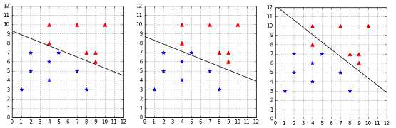
Figure 36: Effect of C=+Infinity, C=1, and C=0.01 on a linearly separable dataset with an outlier

Eventually, in the case where the outlier makes the data non-separable, we cannot use $%FontSize=11 %TeXFontSize=11 \documentclass{article} \pagestyle{empty} \begin{document} \[ C=+\infty \] \end{document}$ because there is no solution meeting all the hard margin constraints. Instead, we test several values of $%FontSize=11 %TeXFontSize=11 \documentclass{article} \pagestyle{empty} \begin{document} \[ C \] \end{document}$ , and we see that the best hyperplane is achieved with $%FontSize=11 %TeXFontSize=11 \documentclass{article} \pagestyle{empty} \begin{document} \[ C=3 \] \end{document}$ . In fact, we get the same hyperplane for all values of $%FontSize=11 %TeXFontSize=11 \documentclass{article} \pagestyle{empty} \begin{document} \[ C \] \end{document}$ greater than or equal to 3. That is because no matter how hard we penalize it, it is necessary to violate the constraint of the outlier to be able to separate the data. When we use a small $%FontSize=11 %TeXFontSize=11 \documentclass{article} \pagestyle{empty} \begin{document} \[ C \] \end{document}$ , as before, more constraints are violated.

Effect of C=3, C=1, and C=0.01 on a non-separable dataset with an outlier

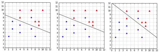
Figure 37: Effect of C=3, C=1, and C=0.01 on a non-separable dataset with an outlier

Rules of thumb:

A small $%FontSize=11 %TeXFontSize=11 \documentclass{article} \pagestyle{empty} \begin{document} \[ C \] \end{document}$ will give a wider margin, at the cost of some misclassifications.
A huge $%FontSize=11 %TeXFontSize=11 \documentclass{article} \pagestyle{empty} \begin{document} \[ C \] \end{document}$ will give the hard margin classifier and tolerates zero constraint violation.
The key is to find the value of $%FontSize=11 %TeXFontSize=11 \documentclass{article} \pagestyle{empty} \begin{document} \[ C \] \end{document}$ such that noisy data does not impact the solution too much.

How to find the best C?

There is no magic value for $%FontSize=11 %TeXFontSize=11 \documentclass{article} \pagestyle{empty} \begin{document} \[ C \] \end{document}$ that will work for all the problems. The recommended approach to select $%FontSize=11 %TeXFontSize=11 \documentclass{article} \pagestyle{empty} \begin{document} \[ C \] \end{document}$ is to use grid search with cross-validation (Hsu, Chang, & Lin, A Practical Guide to Support Vector Classification). The crucial thing to understand is that the value of $%FontSize=11 %TeXFontSize=11 \documentclass{article} \pagestyle{empty} \begin{document} \[ C \] \end{document}$ is very specific to the data you are using, so if one day you found that C=0.001 did not work for one of your problems, you should still try this value with another problem, because it will not have the same effect.

Other soft-margin formulations

2-Norm soft margin

There is another formulation of the problem called the 2-norm (or L2 regularized) soft margin in which we minimize $%FontSize=11 %TeXFontSize=11 \documentclass{article} \pagestyle{empty} \begin{document} $ \frac{1}{2}\|\mathbf{w}\|^2 + C\sum\limits_{i=1}^{m}\zeta_i^2 $ \end{document}$ . This formulation leads to a Wolfe dual problem without the box constraint. For more information about the 2-norm soft margin, refer to (Cristianini & Shawe-Taylor, 2000).

nu-SVM

Because the scale of $%FontSize=11 %TeXFontSize=11 \documentclass{article} \pagestyle{empty} \begin{document} \[ C \] \end{document}$ is affected by the feature space, another formulation of the problem has been proposed: the $%FontSize=11 %TeXFontSize=11 \documentclass{article} \pagestyle{empty} \begin{document} \[ \nuSVM \] \end{document}$ $%FontSize=11 %TeXFontSize=11 \documentclass{article} \pagestyle{empty} \begin{document} \[ \nu SVM \] \end{document}$ . The idea is to use a parameter $%FontSize=11 %TeXFontSize=11 \documentclass{article} \pagestyle{empty} \begin{document} \[ \nu \] \end{document}$ whose value is varied between 0 and 1, instead of the parameter $%FontSize=11 %TeXFontSize=11 \documentclass{article} \pagestyle{empty} \begin{document} \[ C \] \end{document}$ .

Note: “ gives a more transparent parametrization of the problem, which does not depend on the scaling of the feature space, but only on the noise level in the data.” (Cristianini & Shawe-Taylor, 2000)

The optimization problem to solve is:

$%FontSize=11 %TeXFontSize=11 \documentclass{article} \pagestyle{empty} \begin{document} $$ \begin{equation*} \begin{aligned} & \underset{\alpha}{\text{maximize}} & & -\frac{1}{2}\sum\limits_{i=1}^m \sum\limits_{j=1}^m \alpha_i\alpha_j y_i y_j \mathbf{x}_i\cdot \mathbf{x}_j \\ & \text{subject to} & & 0 \leq \alpha_i \leq \frac{1}{m},\\ & & & \sum\limits_{i=1}^m \alpha_i y_i=0 \\ & & & \sum\limits_{i=1}^m \alpha_i \geq \nu \; \text{for any}\ i = 1, \ldots, m \\ \end{aligned} \end{equation*} $$ \end{document}$

Summary

The soft-margin SVM formulation is a nice improvement over the hard-margin classifier. It allows us to classify data correctly even when there is noisy data that breaks linear separability. However, the cost of this added flexibility is that we now have an hyperparameter $%FontSize=11 %TeXFontSize=11 \documentclass{article} \pagestyle{empty} \begin{document} \[ C \] \end{document}$ , for which we need to find a value. We saw how changing the value of $%FontSize=11 %TeXFontSize=11 \documentclass{article} \pagestyle{empty} \begin{document} \[ C \] \end{document}$ impacts the margin and allows the classifier to make some mistakes in order to have a bigger margin. This once again reminds us that our goal is to find a hypothesis that will work well on unseen data. A few mistakes on the training data is not a bad thing if the model generalizes well in the end.