Prerequisites

---

This chapter introduces some basics you need to know in order to understand SVMs better. We will first see what vectors are and look at some of their key properties. Then we will learn what it means for data to be linearly separable before introducing a key component: the hyperplane.

Vectors

In Support Vector Machine, there is the word vector. It is important to know some basics about vectors in order to understand SVMs and how to use them.

What is a vector?

A vector is a mathematical object that can be represented by an arrow (Figure 1).

Figure 1: Representation of a vector

When we do calculations, we denote a vector with the coordinates of its endpoint (the point where the tip of the arrow is). In Figure 1, the point A has the coordinates (4,3). We can write:

If we want to, we can give another name to the vector, for instance, .

From this point, one might be tempted to think that a vector is defined by its coordinates. However, if I give you a sheet of paper with only a horizontal line and ask you to trace the same vector as the one in Figure 1, you can still do it.

You need only two pieces of information:

• What is the length of the vector?
• What is the angle between the vector and the horizontal line?

This leads us to the following definition of a vector:

A vector is an object that has both a magnitude and a direction.

Let us take a closer look at each of these components.

The magnitude of a vector

The magnitude, or length, of a vector  is written , and is called its norm.

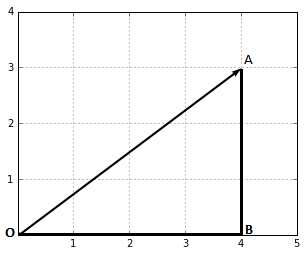
Figure 2: The magnitude of this vector is the length of the segment OA

In Figure 2, we can calculate the norm of vector by using the Pythagorean theorem:

In general, we compute the norm of a vector   by using the Euclidean norm formula: 

In Python, computing the norm can easily be done by calling the norm function provided by the numpy module, as shown in Code Listing 1.

Code Listing 1

The direction of a vector

The direction is the second component of a vector. By definition, it is a new vector for which the coordinates are the initial coordinates of our vector divided by its norm.

The direction of a vector is the vector:

It can be computed in Python using the code in Code Listing 2.

Code Listing 2

Where does it come from? Geometry. Figure 3 shows us a vector and its angles with respect to the horizontal and vertical axis. There is an angle (theta) between and the horizontal axis, and there is an angle (alpha) between and the vertical axis.

Figure 3: A vector u and its angles with respect to the axis

Using elementary geometry, we see that and  , which means that can also be defined by: 

The coordinates of are defined by cosines. As a result, if the angle between and an axis changes, which means the direction of changes, will also change. That is why we call this vector the direction of vector . We can compute the value of (Code Listing 3), and we find that its coordinates are  .

Code Listing 3

It is interesting to note is that if two vectors have the same direction, they will have the same direction vector (Code Listing 4).

Code Listing 4

Moreover, the norm of a direction vector is always 1. We can verify that with the vector (Code Listing 5).

Code Listing 5

It makes sense, as the sole objective of this vector is to describe the direction of other vectors—by having a norm of 1, it stays as simple as possible. As a result, a direction vector such as is often referred to as a unit vector.

Dimensions of a vector

Note that the order in which the numbers are written is important. As a result, we say that a -dimensional vector is a tuple of real-valued numbers.

For instance, is a two-dimensional vector; we often write ( belongs to ).
Similarly, the vector is a three-dimensional vector, and .

The dot product

The dot product is an operation performed on two vectors that returns a number. A number is sometimes called a scalar; that is why the dot product is also called a scalar product.

People often have trouble with the dot product because it seems to come out of nowhere. What is important is that it is an operation performed on two vectors and that its result gives us some insights into how the two vectors relate to each other. There are two ways to think about the dot product: geometrically and algebraically.

Geometric definition of the dot product

Geometrically, the dot product is the product of the Euclidean magnitudes of the two vectors and the cosine of the angle between them.

Figure 4: Two vectors x and y

This means that if we have two vectors,  and , with an angle   between them (Figure 4), their dot product is:

By looking at this formula, we can see that the dot product is strongly influenced by the angle :

• When ,  we have    and 
• When , we have   and 
• When , we have   and 

Keep this in mind—it will be useful later when we study the Perceptron learning algorithm.

We can write a simple Python function to compute the dot product using this definition (Code Listing 6) and use it to get the value of the dot product in Figure 4 (Code Listing 7).

Code Listing 6

However, we need to know the value of to be able to compute the dot product.

Code Listing 7

Algebraic definition of the dot product

Figure 5: Using these three angles will allow us to simplify the dot product

In Figure 5, we can see the relationship between the three angles , (beta), and  (alpha):

This means computing is the same as computing .

Using the difference identity for cosine we get:

If we multiply both sides by  we get:

We already know that:

This means the dot product can also be written:

Or:

In a more general way, for -dimensional vectors, we can write:

This formula is the algebraic definition of the dot product.

Code Listing 8

This definition is advantageous because we do not have to know the angle to compute the dot product. We can write a function to compute its value (Code Listing 8) and get the same result as with the geometric definition (Code Listing 9).

Code Listing 9

Of course, we can also use the dot function provided by numpy (Code Listing 10).

Code Listing 10

We spent quite some time understanding what the dot product is and how it is computed. This is because the dot product is a fundamental notion that you should be comfortable with in order to figure out what is going on in SVMs. We will now see another crucial aspect, linear separability.

Understanding linear separability

In this section, we will use a simple example to introduce linear separability.

Linearly separable data

Imagine you are a wine producer. You sell wine coming from two different production batches:

• One high-end wine costing $145 a bottle.
• One common wine costing $8 a bottle.

Recently, you started to receive complaints from clients who bought an expensive bottle. They claim that their bottle contains the cheap wine. This results in a major reputation loss for your company, and customers stop ordering your wine.

Using alcohol-by-volume to classify wine

You decide to find a way to distinguish the two wines. You know that one of them contains more alcohol than the other, so you open a few bottles, measure the alcohol concentration, and plot it.

Figure 6: An example of linearly separable data

In Figure 6, you can clearly see that the expensive wine contains less alcohol than the cheap one. In fact, you can find a point that separates the data into two groups. This data is said to be linearly separable. For now, you decide to measure the alcohol concentration of your wine automatically before filling an expensive bottle. If it is greater than 13 percent, the production chain stops and one of your employee must make an inspection. This improvement dramatically reduces complaints, and your business is flourishing again.

This example is too easy—in reality, data seldom works like that. In fact, some scientists really measured alcohol concentration of wine, and the plot they obtained is shown in Figure 7. This is an example of non-linearly separable data. Even if most of the time data will not be linearly separable, it is fundamental that you understand linear separability well. In most cases, we will start from the linearly separable case (because it is the simpler) and then derive the non-separable case.

Similarly, in most problems, we will not work with only one dimension, as in Figure 6. Real-life problems are more challenging than toy examples, and some of them can have thousands of dimensions, which makes working with them more abstract. However, its abstractness does not make it more complex. Most examples in this book will be two-dimensional examples. They are simple enough to be easily visualized, and we can do some basic geometry on them, which will allow you to understand the fundamentals of SVMs.

Figure 7: Plotting alcohol by volume from a real dataset

In our example of Figure 6, there is only one dimension: that is, each data point is represented by a single number. When there are more dimensions, we will use vectors to represent each data point. Every time we add a dimension, the object we use to separate the data changes. Indeed, while we can separate the data with a single point in Figure 6, as soon as we go into two dimensions we need a line (a set of points), and in three dimensions we need a plane (which is also a set of points).

To summarize, data is linearly separable when:

• In one dimension, you can find a point separating the data (Figure 6).
• In two dimensions, you can find a line separating the data (Figure 8).
• In three dimensions, you can find a plane separating the data (Figure 9).

Similarly, when data is non-linearly separable, we cannot find a separating point, line, or plane. Figure 10 and Figure 11 show examples of non-linearly separable data in two and three dimensions.

Hyperplanes

What do we use to separate the data when there are more than three dimensions? We use what is called a hyperplane.

What is a hyperplane?

In geometry, a hyperplane is a subspace of one dimension less than its ambient space.

This definition, albeit true, is not very intuitive. Instead of using it, we will try to understand what a hyperplane is by first studying what a line is.

If you recall mathematics from school, you probably learned that a line has an equation of the form , that the constant   is known as the slope, and that intercepts the y-axis. There are several values of for which this formula is true, and we say that the set of the solutions is a line.

What is often confusing is that if you study the function   in a calculus course, you will be studying a function with one variable.

However, it is important to note that the linear equation has two variables, respectively   and , and we can name them as we want.

For instance, we can rename   as   and as , and the equation becomes:  .

This is equivalent to .

If we define the two-dimensional vectors  and , we obtain another notation for the equation of a line (where is the dot product of and ):

What is nice with this last equation is that it uses vectors. Even if we derived it by using two-dimensional vectors, it works for vectors of any dimensions. It is, in fact, the equation of a hyperplane.

From this equation, we can have another insight into what a hyperplane is: it is the set of points satisfying . And, if we keep just the essence of this definition: a hyperplane is a set of points.

If we have been able to deduce the hyperplane equation from the equation of a line, it is because a line is a hyperplane. You can convince yourself by reading the definition of a hyperplane again. You will notice that, indeed, a line is a two-dimensional space surrounded by a plane that has three dimensions. Similarly, points and planes are hyperplanes, too.

Understanding the hyperplane equation

We derived the equation of a hyperplane from the equation of a line. Doing the opposite is interesting, as it shows us more clearly the relationship between the two.

Given vectors , and , we can define a hyperplane having the equation:

This is equivalent to:

We isolate to get:

If we define and :

We see that the bias of the line equation is only equal to the bias of the hyperplane equation when . So you should not be surprised if is not the intersection with the vertical axis when you see a plot for a hyperplane (this will be the case in our next example). Moreover, if and   have the same sign, the slope   will be negative.

Classifying data with a hyperplane

Figure 12: A linearly separable dataset

Given the linearly separable data of Figure 12, we can use a hyperplane to perform binary classification.

For instance, with the vector and we get the hyperplane in Figure 13.

Figure 13: A hyperplane separates the data

We associate each vector   with a label , which can have the value or   (respectively the triangles and the stars in Figure 13).

We define a hypothesis function :

which is equivalent to:

It uses the position of with respect to the hyperplane to predict a value for the label . Every data point on one side of the hyperplane will be assigned a label, and every data point on the other side will be assigned the other label.

For instance, for , is above the hyperplane. When we do the calculation, we get  , which is positive, so  .

Similarly, for  , is below the hyperplane, and will return   because .

Because it uses the equation of the hyperplane, which produces a linear combination of the values, the function , is called a linear classifier.

With one more trick, we can make the formula of even simpler by removing the b constant. First, we add a component to the vector . We get the vector   (it reads “ hat” because we put a hat on ). Similarly, we add a component to the vector , which becomes .

Note: In the rest of the book, we will call a vector to which we add an artificial coordinate an augmented vector.

When we use augmented vectors, the hypothesis function becomes:

If we have a hyperplane that separates the data set like the one in Figure 13, by using the hypothesis function , we are able to predict the label of every point perfectly.
The main question is: how do we find such a hyperplane?

How can we find a hyperplane (separating the data or not)?

Recall that the equation of the hyperplane is in augmented form. It is important to understand that the only value that impacts the shape of the hyperplane is . To convince you, we can come back to the two-dimensional case when a hyperplane is just a line. When we create the augmented three-dimensional vectors, we obtain   and . You can see that the vector contains both and , which are the two main components defining the look of the line. Changing the value of gives us different hyperplanes (lines), as shown in Figure 14.

Figure 14: Different values of w will give you different hyperplanes

Summary

After introducing vectors and linear separability, we learned what a hyperplane is and how we can use it to classify data. We then saw that the goal of a learning algorithm trying to learn a linear classifier is to find a hyperplane separating the data. Eventually, we discovered that finding a hyperplane is equivalent to finding a vector .

We will now examine which approaches learning algorithms use to find a hyperplane that separates the data. Before looking at how SVMs do this, we will first look at one of the simplest learning models: the Perceptron.