Support Vector Machines Succinctly^®
by Alexandre Kowalczyk

CHAPTER 9

Multi-Class SVMs

SVMs are able to generate binary classifiers. However, we are often faced with datasets having more than two classes. For instance, the original wine dataset actually contains data from three different producers. There are several approaches that allow SVMs to work for multi-class classification. In this chapter, we will review some of the most popular multi-class methods and explain where they come from.

For all code examples in this chapter, we will use the dataset generated by Code Listing 41 and displayed in Figure 51.

Code Listing 41

import numpy as np

def load_X():
    return np.array([[1, 6], [1, 7], [2, 5], [2, 8],
                     [4, 2], [4, 3], [5, 1], [5, 2],
                     [5, 3], [6, 1], [6, 2], [9, 4],
                     [9, 7], [10, 5], [10, 6], [11, 6],
                     [5, 9], [5, 10], [5, 11], [6, 9],
                     [6, 10], [7, 10], [8, 11]])

def load_y():
    return np.array([1, 1, 1, 1,
                     2, 2, 2, 2, 2, 2, 2,
                     3, 3, 3, 3, 3,
                     4, 4, 4, 4, 4, 4, 4])

A four classes classification problem

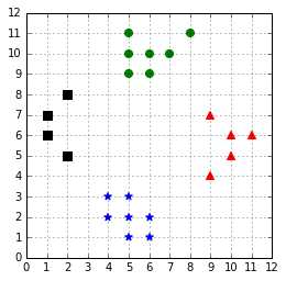
Figure 51: A four classes classification problem

Solving multiple binary problems

One-against-all

Also called “one-versus-the-rest,” this is probably the simplest approach.

In order to classify K classes, we construct K different binary classifiers. For a given class, the positive examples are all the points in the class, and the negative examples are all the points not in the class (Code Listing 42).

Code Listing 42

import numpy as np
from sklearn import svm

# Create a simple dataset

X = load_X()
y = load_y()

# Transform the 4 classes problem

# in 4 binary classes problems.
y_1 = np.where(y == 1, 1, -1)
y_2 = np.where(y == 2, 1, -1)
y_3 = np.where(y == 3, 1, -1)
y_4 = np.where(y == 4, 1, -1)

We train one binary classifier on each problem (Code Listing 43). As a result, we obtain one decision boundary per classifier (in Figure 52).

Code Listing 43

# Train one binary classifier on each problem.
y_list = [y_1, y_2, y_3, y_4]

classifiers = []
for y_i in y_list:
    clf = svm.SVC(kernel='linear', C=1000)
    clf.fit(X, y_i)
    classifiers.append(clf)

The One-against-all approach creates one classifier per class

Figure 52: The One-against-all approach creates one classifier per class

In order to make a new prediction, we use each classifier and predict the class of the classifier if it returns a positive answer (Code Listing 44). However, this can give inconsistent results because a label is assigned to multiple classes simultaneously or to none (Bishop, 2006). Figure illustrates this problem; the one-against-all classifier is not able to predict a class for the examples in the blue areas in each corner because two classifiers are making a positive prediction. This would result in the example having two class simultaneously. The same problem occurs in the center because each classifier makes a negative prediction. As a result, no class can be assigned to an example in this region.

Code Listing 44

def predict_class(X, classifiers):
    predictions = np.zeros((X.shape[0], len(classifiers)))
    for idx, clf in enumerate(classifiers):
        predictions[:, idx] = clf.predict(X)

    # returns the class number if only one classifier predicted it
    # returns zero otherwise.
    return np.where((predictions == 1).sum(1) == 1,
                    (predictions == 1).argmax(axis=1) + 1,
                    0)

One-against-all leads to ambiguous decisions

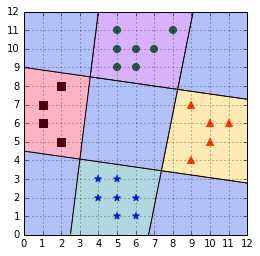
Figure 53: One-against-all leads to ambiguous decisions

As an alternative solution, Vladimir Vapnik suggested using the class of the classifier for which the value of the decision function is the maximum (Vapnik V. N., 1998). This is demonstrated in Code Listing 45. Note that we use the decision_function instead of calling the predict method of the classifier. This method returns a real value that will be positive if the example is on the correct side of the classifier, and negative if it is on the other side. It is interesting to note that by taking the maximum of the value, and not the maximum of the absolute value, this approach will choose the class of the hyperplane the closest to the example when all classifiers disagree. For instance, the example point (6,4) in Figure will be assigned the blue star class.

Code Listing 45

def predict_class(X, classifiers):
    predictions = np.zeros((X.shape[0], len(classifiers)))
    for idx, clf in enumerate(classifiers):
        predictions[:, idx] = clf.decision_function(X)

# return the argmax of the decision function as suggested by Vapnik.
return np.argmax(predictions, axis=1) + 1

Applying this heuristic gives us classification results with no ambiguity, as shown in Figure . The major flaw of this approach is that the different classifiers were trained on different tasks, so there is no guarantee that the quantities returned by the decision_function have the same scale (Bishop, 2006). If one decision function returns a result ten times bigger than results of the others, its class will be assigned incorrectly to some examples.

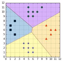
Applying a simple heuristic avoids the ambiguous decision problem

Figure 54: Applying a simple heuristic avoids the ambiguous decision problem

Another issue with the one-against-all approach is that training sets are imbalanced (Bishop, 2006). For a problem with 100 classes, each having 10 examples, each classifier will be trained with 10 positive examples and 990 negative examples. Thus, the negative examples will influence the decision boundary greatly.

Nevertheless, one-against-all remains a popular method for multi-class classification because it is easy to implement and understand.

Note: “[...] In practice the one-versus-the-rest approach is the most widely used in spite of its ad-hoc formulation and its practical limitations.” (Bishop, 2006)

When using sklearn, LinearSVC automatically uses the one-against-all strategy by default. You can also specify it explicitly by setting the multi_class parameter to ovr (one-vs-the-rest), as shown in Code Listing 46.

Code Listing 46

from sklearn.svm import LinearSVC
import numpy as np

X = load_X()
y = load_y()

clf = LinearSVC(C=1000, random_state=88, multi_class='ovr')
clf.fit(X,y)

# Make predictions on two examples.
X_to_predict = np.array([[5,5],[2,5]])
print(clf.predict(X_to_predict)) # prints [2 1]

One-against-one

In this approach, instead of trying to distinguish one class from all the others, we seek to distinguish one class from another one. As a result, we train one classifier per pair of classes, which leads to K(K-1)/2 classifiers for K classes. Each classifier is trained on a subset of the data and produces its own decision boundary (Figure ).

Predictions are made using a simple voting strategy. Each example we wish to predict is passed to each classifier, and the predicted class is recorded. Then, the class having the most votes is assigned to the example (Code Listing 47).

Code Listing 47

from itertools import combinations

from scipy.stats import mode
from sklearn import svm

import numpy as np

# Predict the class having the max number of votes.
def predict_class(X, classifiers, class_pairs):
    predictions = np.zeros((X.shape[0], len(classifiers)))
    for idx, clf in enumerate(classifiers):
        class_pair = class_pairs[idx]
        prediction = clf.predict(X)
        predictions[:, idx] = np.where(prediction == 1,

                                       class_pair[0], class_pair[1])
    return mode(predictions, axis=1)[0].ravel().astype(int)

X = load_X()
y = load_y()

# Create datasets.
training_data = []
class_pairs = list(combinations(set(y), 2))
for class_pair in class_pairs:
    class_mask = np.where((y == class_pair[0]) | (y == class_pair[1]))
    y_i = np.where(y[class_mask] == class_pair[0], 1, -1)
    training_data.append((X[class_mask], y_i))

# Train one classifier per class.
classifiers = []
for data in training_data:
    clf = svm.SVC(kernel='linear', C=1000)
    clf.fit(data[0], data[1])
    classifiers.append(clf)

# Make predictions on two examples.
X_to_predict = np.array([[5,5],[2,5]])
print(predict_class(X_to_predict, classifiers, class_pairs))

# prints [2 1]

One-against-one construct with one classifier for each pair of classes

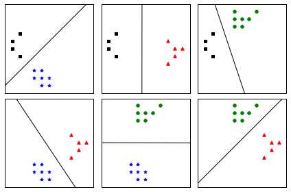
Figure 55: One-against-one construct with one classifier for each pair of classes

With this approach, we are still faced with the ambiguous classification problem. If two classes have an identical number of votes, it has been suggested that selecting the one with the smaller index might be a viable (while probably not the best) strategy (Hsu & Lin, A Comparison of Methods for Multi-class Support Vector Machines, 2002).

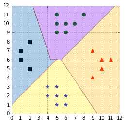
Predictions are made using a voting scheme

Figure 56: Predictions are made using a voting scheme

Figure shows us that the decision regions generated by the one-against-one strategy are different from the ones generated by one-against-all (Figure ). In Figure , it is interesting to note that for regions generated by the one-against-one classifier, a region changes its color only after traversing a hyperplane (denoted by black lines), while this is not the case with one-against-all.

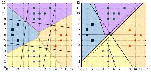
Comparison of one-against-all (left) and one-against-one (right)

Figure 57: Comparison of one-against-all (left) and one-against-one (right)

The one-against-one approach is the default approach for multi-class classification used in sklearn. Instead of Code Listing 47, you will obtain the exact same results using the code of Code Listing 48.

Code Listing 48

from sklearn import svm
import numpy as np

X = load_X()
y = load_y()

# Train a multi-class classifier.
clf = svm.SVC(kernel='linear', C=1000)
clf.fit(X,y)

# Make predictions on two examples.
X_to_predict = np.array([[5,5],[2,5]])
print(clf.predict(X_to_predict)) # prints [2 1]

One of the main drawbacks of the one-against-all method is that the classifier will tend to overfit.
Moreover, the size of the classifier grows super-linearly with the number of classes, so this method will be slow for large problems (Platt, Cristianini, & Shawe-Taylor, 2000).

DAGSVM

DAGSVM stands for “Directed Acyclic Graph SVM.” It has been proposed by John Platt et al. in 2000 as an improvement of one-against-one (Platt, Cristianini, & Shawe-Taylor, 2000).

Note: John C. Platt invented the SMO algorithm and Platt Scaling, and proposed the DAGSVM. Quite a contribution to the SVMs world!

The idea behind DAGSVM is to use the same training as one-against-one, but to speed up testing by using a directed acyclic graph (DAG) to choose which classifiers to use.

If we have four classes A, B, C, and D, and six classifiers trained each on a pair of classes: (A, B); (A, C); (A, D); (B, C); (B, D); and (C, D). We use the first classifier, (A, D), and it predicts class A, which is the same as predicting not class D, and the second classifier also predits class A (not class C). It means that classifiers (B, D), (B, C) or (C, D) can be ignored because we already know the class is neither C nor D. The last “useful” classifier is (A, B), and if it predicts B, we assign the class B to the data-point. This example is illustrated with the red path in Figure . Each node of the graph is a classifier for a pair of class.

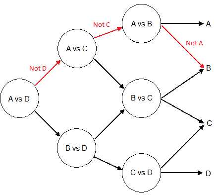
Illustration of the path used to make a prediction along a Directed Acyclic graph

Figure 58: Illustration of the path used to make a prediction along a Directed Acyclic graph

With four classes, we used three classifiers to make the prediction, instead of six with one-against-one. In general, for a problem with K classes, K-1 decision nodes will be evaluated.

Substituting the predict_class function in Code Listing 47 with the one in Code Listing 49 gives the same result, but with the benefit of using fewer classifiers.

In Code Listing 49, we implement the DAGSVM approach with a list. We begin with the list of possible classes, and after each prediction, we remove the one that has been disqualified. In the end, the remaining class is the one which should be assigned to the example.

Note that Code Listing 49 is here for illustration purposes and should not be used in your production code, as it is not fast when the dataset (X) is large.

Code Listing 49

def predict_class(X, classifiers, distinct_classes, class_pairs):
    results = []
    for x_row in X:

        class_list = list(distinct_classes)

        # After each prediction, delete the rejected class
        # until there is only one class.
        while len(class_list) > 1:
            # We start with the pair of the first and

            # last element in the list.
            class_pair = (class_list[0], class_list[-1])
            classifier_index = class_pairs.index(class_pair)
            y_pred = classifiers[classifier_index].predict(x_row)

            if y_pred == 1:
                class_to_delete = class_pair[1]
            else:
                class_to_delete = class_pair[0]

            class_list.remove(class_to_delete)

        results.append(class_list[0])
    return np.array(results)

Note: “The DAGSVM is between a factor 1.6 and 2.3 times faster to evaluate than Max Wins.” (Platt, Cristianini, & Shawe-Taylor, 2000).

Solving a single optimization problem

Instead of trying to solve several binary optimization problems, another approach is to try to solve a single optimization problem. This approach has been proposed by several people over the years.

Vapnik, Weston, and Watkins

This method is a generalization of the SVMs optimization problem to solve the multi-class classification problem directly. It has been independently discovered by Vapnik (Vapnik V. N., 1998) and Weston & Watkins (Weston & Watkins, 1999). For every class, constraints are added to the optimization problem. As a result, the size of the problem is proportional to the number of classes and can be very slow to train.

Crammer and Singer

Crammer and Singer (C&S) proposed an alternative approach to multi-class SVMs. Like Weston and Watkins, they solve a single optimization problem, but with fewer slack variables (Crammer & Singer, 2001). This has the benefit of reducing the memory and training time. However, in their comparative study, Hsu & Lin found that the C&S method was especially slow when using a large value for the C regularization parameter (Hsu & Lin, A Comparison of Methods for Multi-class Support Vector Machines, 2002).

In sklearn, when using LinearSVC you can choose to use the C&S algorithm (Code Listing 50). In Figure , we can see that the C&S predictions are different from the one-against-all and the one-against-one methods.

Code Listing 50

from sklearn import svm
import numpy as np

X = load_X()
y = load_y()

clf = svm.LinearSVC(C=1000, multi_class='crammer_singer')
clf.fit(X,y)

# Make predictions on two examples.
X_to_predict = np.array([[5,5],[2,5]])
print(clf.predict(X_to_predict)) # prints [4 1]

Crammer & Singer algorithm predictions

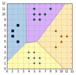
Figure 59: Crammer & Singer algorithm predictions

Which approach should you use?

With so many options available, choosing which multi-class approach is better suited for your problem can be difficult.

Hsu and Lin wrote an interesting paper comparing the different multi-class approaches available for SVMs (Hsu & Lin, A Comparison of Methods for Multi-class Support Vector Machines, 2002). They conclude that “the one-against-one and DAG methods are more suitable for practical use than the other methods.” The one-against-one method has the added advantage of being already available in sklearn, so it should probably be your default choice.

Be sure to remember that LinearSVC uses the one-against-all method by default, and that maybe using the Crammer & Singer algorithm will better help you achieve your goal. On this topic, Dogan et al. found that despite being considerably faster than other algorithms, one-against-all yield hypotheses with a statistically significantly worse accuracy (Dogan, Glasmachers, & Igel, 2011). Table 1 provides an overview of the methods presented in this chapter to help you make a choice.

Table 1: Overview of multi-class SVM methods

Method name	One-against-all	One-against-one	Weston and Watkins	DAGSVM	Crammer and Singer
First SVMs usage	1995	1996	1999	2000	2001
Approach	Use several binary classifiers	Use several binary classifiers	Solve a single optimization problem	Use several binary classifiers	Solve a single optimization problem
Training approach	Train a single classifier for each class	Train a classifier for each pair of classes	Decomposition method	Same as one-against-one	Decomposition method
Number of trained classifiers ( $%FontSize=11 %TeXFontSize=11 \documentclass{article} \pagestyle{empty} \begin{document} \[ K \] \end{document}$ is the number of classes)	$%FontSize=11 %TeXFontSize=11 \documentclass{article} \pagestyle{empty} \begin{document} \[ K \] \end{document}$	$%FontSize=11 %TeXFontSize=11 \documentclass{article} \pagestyle{empty} \begin{document} \[ \frac{K(K-1)}{2} \] \end{document}$	1	$%FontSize=11 %TeXFontSize=11 \documentclass{article} \pagestyle{empty} \begin{document} \[ \frac{K(K-1)}{2} \] \end{document}$	1
Testing approach	Select the class with the biggest decision function value	“Max-Wins” voting strategy	Use the classifier	Use a DAG to make predictions on K-1 classifiers	Use the classifier
scikit-learn class	LinearSVC	SVC	Not available	Not available	LinearSVC
Drawbacks	Class imbalance	Long training time for large K	Long training time	Not available in popular libraries	Long training time

Summary

Thanks to many improvements over the years, there are now several methods for doing multi-class classification with SVMs. Each approach has advantages and drawbacks, and most of the time you will end up using the one available in the library you are using. However, if necessary, you now know which method can be more helpful to solve your specific problem.

Research on multi-class SVMs is not over. Recent papers on the subject have been focused on distributed training. For instance, Han & Berg have presented a new algorithm called “Distributed Consensus Multiclass SVM,” which uses consensus optimization with a modified version of Crammer & Singer’s formulation (Han & Berg, 2012).

Build apps 2X faster

using Syncfusion Essential Studio^® suite

1800+ high-performance UI components.
Includes popular controls such as Grid, Chart, Scheduler, and more.
24x5 unlimited support by developers.

Get Your Free Trial Now