Kernels

Feature transformations

Can we classify non-linearly separable data?

Imagine you have some data that is not separable (like the one in Figure 38), and you would like to use SVMs to classify it. We have seen that it is not possible because the data is not linearly separable. However, this last assumption is not correct. What is important to notice here is that the data is not linearly separable in two dimensions.

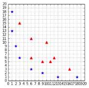
Figure 38: A straight line cannot separate the data

Even if your original data is in two dimensions, nothing prevents you from transforming it before feeding it into the SVM. One possible transformation would be, for instance, to transform every two-dimensional vector into a three-dimensional vector.

For example, we can do what is called a polynomial mapping by applying the function defined by:

Code Listing 31 shows this transformation implemented in Python.

Code Listing 31

If you transform the whole data set of Figure 38 and plot the result, you get Figure 39, which does not show much improvement. However, after some time playing with the graph, we can see that the data is, in fact, separable in three dimensions (Figure 40 and Figure 41)!

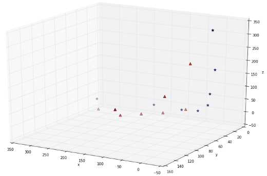
Figure 39: The data does not look separable in three dimensions

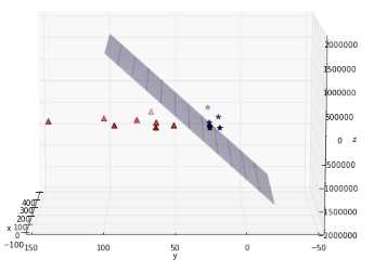
Figure 40: The data is, in fact, separable by a plane

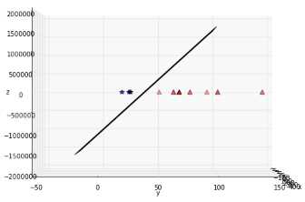
Figure 41: Another view of the data showing the plane from the side

Here is a basic recipe we can use to classify this dataset:

1. Transform every two-dimensional vector into a three-dimensional vector using the transform method of Code Listing 31.
2. Train the SVMs using the 3D dataset.
3. For each new example we wish to predict, transform it using the transform method before passing it to the predict method.

Of course, you are not forced to transform the data into three dimensions; it could be five, ten, or one hundred dimensions.

How do we know which transformation to apply?

Choosing which transformation to apply depends a lot on your dataset. Being able to transform the data so that the machine learning algorithm you wish to use performs at its best is probably one key factor of success in the machine learning world. Unfortunately, there is no perfect recipe, and it will come with experience via trial and error. Before using any algorithm, be sure to check if there are some common rules to transform the data detailed in the documentation. For more information about how to prepare your data, you can read the dataset transformation section on the scikit-learn website.

What is a kernel?

In the last section, we saw a quick recipe to use on the non-separable dataset. One of its main drawbacks is that we must transform every example. If we have millions or billions of examples and that transform method is complex, that can take a huge amount of time. This is when kernels come to the rescue.

If you recall, when we search for the KKT multipliers in the Wolfe dual Lagrangian function, we do not need the value of a training example ; we only need the value of the dot product    between two training examples:

In Code Listing 32, we apply the first step of our recipe. Imagine that when the data is used to learn, the only thing we care about is the value returned by the dot product, in this example 8,100.

Code Listing 32

The question is this: Is there a way to compute this value, without transforming the vectors?

And the answer is: Yes, with a kernel!

Let us consider the function in Code Listing 33:

Code Listing 33

Using this function with the same two examples as before returns the same result (Code Listing 33).

Code Listing 34

When you think about it, this is pretty incredible.

The vectors and belong to . The kernel function computes their dot product as if they have been transformed into vectors belonging to , and it does that without doing the transformation, and without computing their dot product!

To sum up: a kernel is a function that returns the result of a dot product performed in another space. More formally, we can write:

Definition: Given a mapping function  , we call the function defined by ,  where    denotes an inner product in , a kernel function.

The kernel trick

Now that we know what a kernel is, we will see what the kernel trick is.

If we define a kernel as: , we can then rewrite the soft-margin dual problem:

That’s it. We have made a single change to the dual problem—we call it the kernel trick.

Tip: Applying the kernel trick simply means replacing the dot product of two examples by a kernel function.

This change looks very simple, but remember that it took a serious amount of work to derive the Wolf dual formulation from the original optimization problem. We now have the power to change the kernel function in order to classify non-separable data.

Of course, we also need to change the hypothesis function to use the kernel function:

Remember that in this formula is the set of support vectors. Looking at this formula, we better understand why SVMs are also called sparse kernel machines. It is because they only need to compute the kernel function on the support vectors and not on all the vectors, like other kernel methods (Bishop, 2006).

Kernel types

Linear kernel

This is the simplest kernel. It is simply defined by:

where and are two vectors.

In practice, you should know that a linear kernel works well for text classification.

Polynomial kernel

We already saw the polynomial kernel earlier when we introduced kernels, but this time we will consider the more generic version of the kernel:

It has two parameters: , which represents a constant term, and , which represents the degree of the kernel. This kernel can be implemented easily in Python, as shown in Code Listing 35.

Code Listing 35

In Code Listing 36, we see that it returns the same result as the kernel of Code Listing 33 when we use the degree 2. The result of training a SVM with this kernel is shown in Figure 42.

Code Listing 36

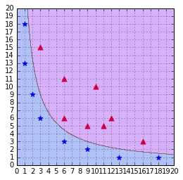
Figure 42: A SVM using a polynomial kernel is able to separate the data (degree=2)

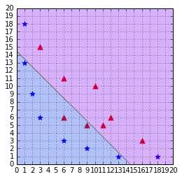
Updating the degree

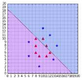
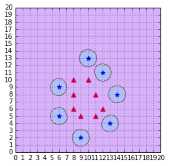
A polynomial kernel with a degree of 1 and no constant is simply the linear kernel (Figure 43). When you increase the degree of a polynomial kernel, the decision boundary will become more complex and will have a tendency to be influenced by individual data examples, as illustrated in Figure 44. Using a high-degree polynomial is dangerous because you can often achieve better performance on your test set, but it leads to what is called overfitting: the model is too close to the data and does not generalize well.

Note: Using a high-degree polynomial kernel will often lead to overfitting.

RBF or Gaussian kernel

Sometimes polynomial kernels are not sophisticated enough to work. When you have a difficult dataset like the one depicted in Figure 45, this type of kernel will show its limitation.

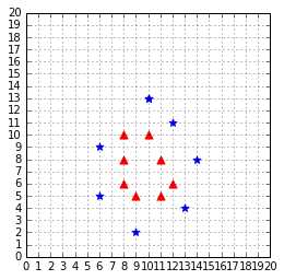
Figure 45: This dataset is more difficult to work with

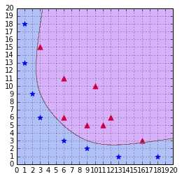
As we can see in Figure 46, the decision boundary is very bad at classifying the data.

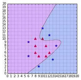
Figure 46: A polynomial kernel is not able to separate the data (degree=3, C=100)

This case calls for us to use another, more complicated, kernel: the Gaussian kernel. It is also named RBF kernel, where RBF stands for Radial Basis Function. A radial basis function is a function whose value depends only on the distance from the origin or from some point.

The RBF kernel function is:

You will often read that it projects vectors into an infinite dimensional space. What does this mean?

Recall this definition: a kernel is a function that returns the result of a dot product performed in another space.

In the case of the polynomial kernel example we saw earlier, the kernel returned the result of a dot product performed in . As it turns out, the RBF kernel returns the result of a dot product performed in .

I will not go into details here, but if you wish, you can read this proof to better understand how we came to this conclusion.

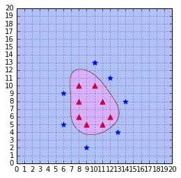
Figure 47: The RBF kernel classifies the data correctly with gamma = 0.1

This video is particularly useful to understand how the RBF kernel is able to separate the data.

Changing the value of gamma

When gamma is too small, as in Figure 48, the model behaves like a linear SVM. When gamma is too large, the model is too heavily influenced by each support vector, as shown in Figure 49. For more information about gamma, you can read this scikit-learn documentation page.

Other types

Research on kernels has been prolific, and there are now a lot of kernels available. Some of them are specific to a domain, such as the string kernel, which can be used when working with text. If you want to discover more kernels, this article from César Souza describes 25 kernels.

Which kernel should I use?

The recommended approach is to try a RBF kernel first, because it usually works well. However, it is good to try the other types of kernels if you have enough time to do so. A kernel is a measure of the similarity between two vectors, so that is where domain knowledge of the problem at hand may have the biggest impact. Building a custom kernel can also be a possibility, but it requires that you have a good mathematical understanding of the theory behind kernels. You can find more information on this subject in (Cristianini & Shawe-Taylor, 2000).

Summary

The kernel trick is one key component making Support Vector Machines powerful. It allows us to apply SVMs on a wide variety of problems. In this chapter, we saw the limitations of the linear kernel, and how a polynomial kernel can classify non-separable data. Eventually, we saw one of the most used and most powerful kernels: the RBF kernel. Do not forget that there are many kernels, and try looking for kernels created to solve the kind of problems you are trying to solve. Using the right kernel with the right dataset is one key element in your success or failure with SVMs.