
Statistics Using Excel Succinctly®

CHAPTER 7
Student’s t Distribution
Basic Concepts
The one sample hypothesis test using the normal distribution as described in chapter 5, is fine when one knows the standard deviation of the population distribution and the population is either normally distributed or the sample is sufficiently large that the Central Limit Theorem applies.
The problem with this approach is that the standard deviation of the population is generally not known. One way of addressing this is to use the standard deviation s of the sample instead of the standard deviation σ of the population employing the t distribution.
The (Student’s) t distribution with k degrees of freedom has probability density function given by the formula
fx= Γk+12πkΓk21+x2k-(k+1)2
where Γ(x) is the gamma function.
The overall shape of the probability density function of the t distribution resembles the bell shape of a normally distribution with mean 0 and variance 1, except that it is a bit lower and wider. As the number of degrees of freedom grows, the t distribution approaches the standard normal distribution, and in fact the approximation is quite close for k ≥ 30.

- Chart of the t distribution by degrees of freedom
If x has a normal distribution with mean μ and standard deviation σ then for samples of size n, the random variable
t=x-μsn
has a t distribution with n – 1 degrees of freedom. The same is true even when x doesn’t have a normal distribution provided that n is sufficiently large (by the Central Limit Theorem).
This test statistic is the same as z=x-μσn from the Central Limit Theorem with the population standard deviation σ replaced by the sample standard deviation s. What makes this useful is that usually the standard deviation of the population is unknown while the standard deviation of the sample is known.
Excel Functions
Excel provides the T.DIST, T.INV, T.DIST.RT, T.INV.RT and T.INV.2T functions to calculate values for the t distribution and its inverse. These functions were not available prior to Excel 2007. The following table lists how these functions are used as well as their equivalents using the functions TDIST and TINV which were used prior to Excel 2007.
Table 8: Excel t distribution functions
Tail | Distribution | Inverse |
|---|---|---|
Right tail | T.DIST.RT(x, df) = TDIST(x, df, 1) | T.INV(1-α, df) = TINV(2*α, df) |
Left tail | T.DIST(x, df, TRUE) = TDIST(-x, df, 1) | T.INV(α, df) = -TINV(2*α, df) |
Two tail | T.DIST.2T(x, df) = TDIST(x, df, 2) | T.INV.2T(α, df) = TINV(α, df) |
T.DIST has two forms. T.DIST(x, df, TRUE) is the value of the cumulative t distribution function with df degrees of freedom at x, while T.DIST(x, df, FALSE) is the value of the probability density function at x.
Hypothesis Testing
One Sample Testing
As explained previously, the t distribution provides a good way to perform one sample tests on the mean when the population variance is not known provided the population is normal or the sample is sufficiently large so that the Central Limit Theorem applies.
It turns out that the t distribution provides good results even when the population is not normal and even when the sample is small, provided the sample data is reasonably symmetrically distributed about the sample mean. This can be determined by graphing the data. The following are indications of symmetry:
- The boxplot is relatively symmetrical; i.e. the median is in the center of the box and the whiskers extend equally in each direction
- The histogram looks symmetrical
- The mean is approximately equal to the median
- The coefficient of skewness is relatively small
Example: A weight reduction program claims to be effective in treating obesity. To test this claim 12 people were put on the program and the number of pounds of weight gain/loss was recorded for each person after two years, as shown in columns A and B of Figure 32. Can we conclude that the program is effective?

- One sample t test
A negative value in column B indicates that the subject gained weight. We judge the program to be effective if there is some weight loss at the 95% significance level. We choose to conduct a two-tailed test since there is risk that the program might actual result in weight gain rather than loss. Thus our null hypothesis is:
H0: μ = 0; i.e. the program is not effective
From the box plot in Figure 33 we see that the data is quite symmetric and so we use the t test even though the sample is small.

- Box plot of the sample data
Column E of Figure 33 contains all the formulas required to carry out the t test. Since Excel only displays the values of these formulas, we show each of the formulas (in text format) in column G so that you can see how the calculations are performed.
Thus where R is B4:B15, we see that n = COUNT(R) = 12, x = AVERAGE(R) = 5.5, s = STDEV(R) = 11.42 and standard error = sn = 3.30. From this we see that
t= x-μsn= 5.5-03.3=1.668 with df = 11 degrees of freedom
Since p-value = T.DIST.2T(t, df) = T.DIST.2T(1.668, 11) = .123 > .05 = α, the null hypothesis is not rejected. This means there is an 12.3% probability of achieving a value for t this high assuming that the null hypothesis is true, and since 12.3% > 5% we can’t reject the null hypothesis.
The same conclusion is reached since
t-crit = T.INV.2T(α, df) = T.INV.2T(.05, 11) = 2.20 > 1.668 = t-obs
Here we used T.DIST.2T and T.INV.2T since we are using a two-tailed test.
Testing Two Independent Samples
Assuming equal population variances
Our goal is to determine whether the means of two populations are equal given two independent samples, one from each population. We start by assuming that population variances are equal even if unknown.
Suppose that x and y are the sample means of two independent samples of size nx and ny respectively, and suppose that sx and sy are the sample standard deviations of two sets of data. If x and y are normal or if nx and ny are sufficiently large for the Central Limit Theorem to hold, then the statistic
t= x-y-μx-μys1nx+1ny
has a t distribution with nx+ny-2 degrees of freedom where s2 is the pooled variance defined by
s2= nx-1sx2+ny-1sy2(nx-1)+(ny -1)
We can use t to test the null hypothesis that the two population means are equal, or equivalently that μx-μy=0. It turns out that even when x and y are not normal and nx and ny are not particularly large, as long as the two samples are reasonably symmetric then this test yields pretty good results.
Example: A food company wants to determine whether their new formula for peanut butter is significantly tastier than their old formula. They chose two random samples of ten people and asked the people in the first sample to taste the peanut butter using the existing formula and the people in the second sample to taste the peanut butter with the new formula. They then asked all twenty people to fill out a questionnaire rating the tastiness of the peanut butter they tasted.
Based on the data in Figure 34, determine whether there is a significant difference between the two types of peanut butter.
As we can see from Figure 34 the mean score for the new formula is 15, while the mean score for the old formula is 11, but is this difference just due to random effects or is there a statistically significant difference?
We also note that the variances for the two samples are 13.3 and 18.8. It turns out that these two values are close enough to satisfy the equal variance assumption.

- Sample data
Finally if we draw the box plots for the two data sets we see that both are relatively symmetric (i.e. for each sample the colored areas in each box are approximately equal in size and the upper and lower whiskers are fairly equal in length).
Thus the assumptions for the t test are met. To carry out the test we use Excel’s t-Test: Two Sample Assuming Equal Variances data analysis tool, which, as usual can be accessed by selecting Data > Analysis|Data Analysis. The result is shown in Figure 35.
t-Test: Two-Sample Assuming Equal Variances | ||
| New | Old |
Mean | 15 | 11.1 |
Variance | 13.33333 | 18.76667 |
Observations | 10 | 10 |
Pooled Variance | 16.05 | |
Hypothesized Mean Difference | 0 | |
df | 18 | |
t Stat | 2.176768 | |
P(T<=t) one-tail | 0.021526 | |
t Critical one-tail | 1.734064 | |
P(T<=t) two-tail | 0.043053 | |
t Critical two-tail | 2.100922 |
|
- Two sample t test assuming equal variance
Assuming that we are performing a two-tailed test, we see that the p-value = 0.043 which is less than the usual alpha value of .05, and so we conclude that there is a significant difference between the mean scores for the two peanut butter formulations.
Assuming unequal population variances
In the previous section we assumed that the two population variances were equal (or at least not very unequal). When the assumptions of equal populations variance is not met (or when we don’t have enough evidence to draw this conclusion) we can modify the approach used in the previous section by employing a slightly different version of the t test.
Suppose that x and y are the sample means of two independent samples of size nx and ny respectively, and suppose that sx and sy are the sample standard deviations of the two sets of data. If x and y are normal or if nx and ny are sufficiently large for the Central Limit Theorem to hold, then the statistic
t= x-y-μx-μysx2nx+sy2ny
has a t distribution with the following degrees of freedom.
df= sx2nx+sy2ny2sx2nx2nx-1+sy2ny2ny-1
Example: Repeat the previous analysis using the data in Figure 36.

- Revised sample data
This time we see that there is a big difference between the variances (118.3 vs. 18.8).
Generally, even if one variance is up to 4 times the other, the equal variance assumption will give good results. This rule of thumb is clearly violated in this example and so we need to use the t test with unequal population variances, namely Excel’s t-Test: Two Sample Assuming Unequal Variances data analysis tool.
The output is shown in Figure 37.
t-Test: Two-Sample Assuming Unequal Variances | ||
| New | Old |
Mean | 18.9 | 11.1 |
Variance | 118.3222 | 18.76667 |
Observations | 10 | 10 |
Hypothesized Mean Difference | 0 | |
df | 12 | |
t Stat | 2.106655 | |
P(T<=t) one-tail | 0.028434 | |
t Critical one-tail | 1.782288 | |
P(T<=t) two-tail | 0.056869 | |
t Critical two-tail | 2.178813 |
|
- Two sample t test assuming unequal variance
Note that the degrees of freedom have been reduced from 18 in Example 1 to 12 in this example (actually 11.78, although Excel rounds this up to 12). Since for the two-tail test, p-value = 0.056869 > .05 = α, we cannot reject the null hypothesis that there is no significant difference between the two formulations.
If we had used the equal variance test we would have gotten the results shown in Figure 6, which would have led us to a different conclusion since for the two-tail test p-value = 0.049441 < .05 = α, and we would have concluded that there was a significant difference between the two formulations.
t-Test: Two-Sample Assuming Equal Variances | ||
| New | Old |
Mean | 18.9 | 11.1 |
Variance | 118.3222 | 18.76667 |
Observations | 10 | 10 |
Pooled Variance | 68.54444 | |
Hypothesized Mean Difference | 0 | |
df | 18 | |
t Stat | 2.106655 | |
P(T<=t) one-tail | 0.024721 | |
t Critical one-tail | 1.734064 | |
P(T<=t) two-tail | 0.049441 | |
t Critical two-tail | 2.100922 |
|
- Same problem assuming equal variance
Testing Paired Samples
In paired sample hypothesis testing, a sample from the population is chosen and two measurements for each element in the sample are taken. Each set of measurements is considered a sample. Unlike the hypothesis testing studied so far, the two samples are not independent of one another.
For example, if you want to determine whether drinking a glass of wine or drinking a glass of beer has the same or different impact on memory, one approach is to take a sample of say 40 people, and have half of them drink a glass of wine and the other half drink a glass of beer, and then give each of the 40 people a memory test and compare results. This is the approach with independent samples.
Another approach is to take a sample of 20 people and have each person drink a glass of wine and take a memory test, and then have the same people drink a glass of beer and again take a memory test; finally we compare the results. This is the approach used with paired samples.
The advantage of this second approach is the sample can be smaller. Also since the sampled subjects are the same for beer and wine there is less chance that some external factor (confounding variable) will influence the result. The problem with this approach is that it is possible that the results of the second memory test will be lower simply because the person has imbibed more alcohol. This can be corrected by sufficiently separating the tests, e.g., by conducting the test with beer a day after the test with wine.
It is also possible that the order in which people take the tests influences the result (e.g., the subjects learn something on the first test that helps them on the second test, or perhaps taking the test the second time introduces a degree of boredom that lowers the score). One way to address these order effects is to have half the people drink wine on day 1 and beer on day 2, while for the other half the order is reversed (called counterbalancing).
Obviously not all experiments can use the paired sample design. E.g., if you are testing differences between men and women, then independent samples will be necessary.
Example: A clinic provides a program to help their clients lose weight and asks a consumer agency to investigate the effectiveness of the program. The agency takes a sample of 15 people, weighing each person in the sample before the program begins and 3 months later to produce the table in Figure 39. Determine whether the program is effective.
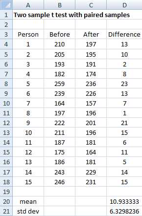
- Sample data
The program is effective if there is a significant reduction in the weight of the people in the program. Let x = the difference in weight 3 months after the program starts. The null hypothesis is:
H0: μ = 0; i.e. any differences in weight is due to chance
Essentially the test to use is the one sample test, as described previously, but on the difference in the weight before the program minus the weight after the program. Since all the values in column D of Figure 39 are positive, we see that all the subjects in the sample lost weight, but is the reduction significant?
We could create the analysis as in Figure 32 using column D of Figure 39 as the single sample. Instead, we will use Excel’s t-Test: Paired Two Sample for Means data analysis tool. We begin by selecting Data > Analysis|Data Analysis.
When the dialog box shown in Figure 40 appears, you need to fill in the values as shown in the figure and click on the OK button.

- T-Test: Paired Two Sample for Means dialog box
The output of the analysis is displayed in Figure 41.
t-Test: Paired Two Sample for Means | ||
| Before | After |
Mean | 207.9333 | 197 |
Variance | 815.781 | 595 |
Observations | 15 | 15 |
Pearson Correlation | 0.98372 | |
Hypothesized Mean Difference | 0 | |
df | 14 | |
t Stat | 6.6897 | |
P(T<=t) one-tail | 5.14E-06 | |
t Critical one-tail | 1.76131 | |
P(T<=t) two-tail | 1.03E-05 | |
t Critical two-tail | 2.144787 |
|
- Paired sample t-test analysis
Since the p-value for the two-tail test is 1.03E-05, we conclude that there is a significant difference between the mean weights. Since the mean after is lower than the mean weight before, we can conclude that there is a significant reduction in weight, and so it is fair to say that the program is effective (at least for the 3 month period).
Using the T.TEST Function
In addition to the approaches shown in the last few sections, Excel provides the T.TEST function to perform the three different types of two sample t tests.
T.TEST(R1, R2, tails, type) = the t-test value for the difference between the means of two samples R1 and R2, where tails = 1 (one-tailed) or 2 (two-tailed) and type takes the values:
- the samples have paired values from the same population
- the samples are from populations with the same variance
- the samples are from populations with different variances
These three types correspond to the Excel data analysis tools
- t-Test: Paired Two Sample for Mean
- t-Test: Two-Sample Assuming Equal Variance
- t-Test: Two-Sample Assuming Unequal Variance
The T.TEST function is not available for versions of Excel prior to Excel 2010. For earlier versions of Excel the TTEST function is available which provides identical functionality.
By way of example, we repeat the analysis from Figure 35 using the T.TEST function. As we can see from Figure 42, the p-value for the two-tailed test for two independent samples from populations with the same variances is 0.043053 (cell E40). This is the same as the result found previously.

- T.TEST for two independent samples
Figure 42 also shows the value of the test if we didn’t assume equal variances (cell 39). As you can see, there is very little difference between the two results.
Confidence Intervals
Until now, we have made what are called point estimates of the mean or differences between means. We now define the confidence interval, which provides a range of possible values instead of just a single measurement. We illustrate how this works using the t distribution.
The 1 – α confidence interval for the population mean is
observed mean ±tcrit∙std error
Example: Calculate the 95% confidence interval for the one sample t test example (see Figure 32).
meanobs±tcrit∙std err=5.5 ±2.201 ∙3.297=5.5± 7.257
This yields a 95% confidence interval of (-1.757, 12.757) for the population mean. Since the interval contains the hypothetical mean of 0, once again we are justified in our conclusion not to reject the null hypothesis.
Version of Excel starting with Excel 2010 provide the following function to calculate the confidence interval for the t distribution.
CONFIDENCE.T(α, s, n) = k such that ( x – k, x + k) is the 1 – α confidence interval for the population mean; i.e. CONFIDENCE.T(α, s, n) = tcrit ∙ std error, where n = sample size and s = sample standard deviation.
Thus for the last example, we calculate CONFIDENCE.T(.05,11.422,12) = 7.257 which yields a 95% confidence interval of 5.5± 7.257, as before.
- 1800+ high-performance UI components.
- Includes popular controls such as Grid, Chart, Scheduler, and more.
- 24x5 unlimited support by developers.