Normal Distribution

---

Normal Distribution

Basic Concepts

The probability density function of the normal distribution is defined by:

fx= 1σ2πe-12x-μσ2

where e is the constant 2.7183..., and π is the constant 3.1415…

The normal distribution is completely determined by the parameters μ and σ. It turns out that μ is the mean of the normal distribution and σ is the standard deviation.

The graph of the normal distribution has the shape of a bell curve, as shown in Figure 25.

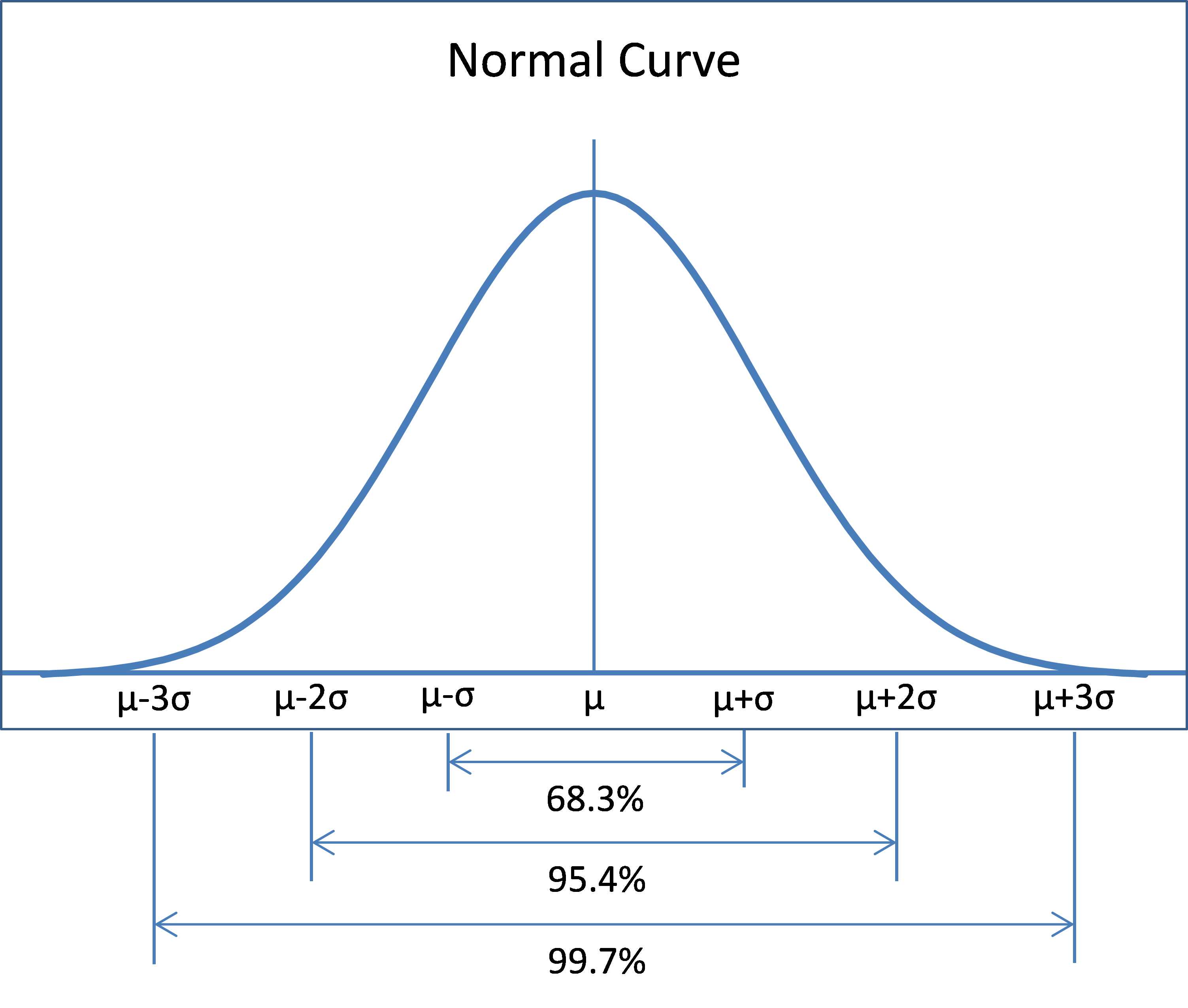
25. Normal Curve

Some characteristics of the normal distribution are as follows:

• Mean = median = mode = μ
• Standard deviation = σ
• Skewness = kurtosis = 0

The function is symmetric about the mean with inflection points (i.e. the points where there curve changes from concave up to concave down or from concave down to concave up) at x=μ±σ.

As can be seen from Figure 25, the area under the curve in the interval μ –σ<x<μ+σ is approximately 68.26% of the total area under the curve. The area under the curve in the interval μ –2σ<x<μ+2σ is approximately 95.44% of the total area under the curve and the area under the curve in the interval μ –3σ<x<μ+3σ is approximately 99.74% of the area under the curve.

As we shall see, the normal distribution occurs frequently and is very useful in statistics.

Excel Functions

Excel provides the following functions regarding the normal distribution:

      NORM.DIST(x, μ, σ, cum) where cum takes the values TRUE and FALSE.

NORMDIST(x, μ, σ, FALSE) = probability density function value at x for the normal distribution with mean μ and standard deviation σ.

NORMDIST(x, μ, σ, TRUE) = cumulative probability distribution function value at x for the normal distribution with mean μ and standard deviation σ.

NORM.INV(p, μ, σ) is the inverse of NORMDIST(x, μ, σ, TRUE), i.e.

NORMINV(p, μ, σ) = the value x such that NORMDIST(x, μ, σ, TRUE) = p

These functions are not available in versions of Excel prior to Excel 2010. Instead these versions of Excel provide NORMDIST, which is equivalent to NORM.DIST and NORMINV, which is equivalent to NORM.INV.

Example

Create a graph of the distribution of IQ scores using the Stanford-Binet scale.

This distribution is known to have a normal distribution with mean 100 and standard deviation 16. To create the graph, we first create a table with the values of the probability density function f(x) for x = 50, 51, …, 150. This table begins as shown on the left side of Figure 26.

26. Distribution of IQ scores

We only show the first 20 entries, but in total there are 101 entries occupying the range A4:B104. The values in column B are calculated using the NORM.DIST function. E.g., the formula in cell B4 is

      =NORM.DIST(A4,100,16,FALSE)

We can draw the chart on the right side of Figure 26 by highlighting the range B4:B104 and then selecting Insert > Charts|Line. The display of the chart can be improved as described elsewhere in this book.

Standard Normal Distribution

The standard normal distribution is a normal distribution with a mean of 0 and a standard deviation of 1.

To convert a random variable x with normal distribution with mean μ and standard deviation σ to standard normal form you use the following linear transformation:

z= x-μ σ

The resulting random variable is called a z-score. Excel provides the following function for calculating the value of z from x, μ and σ.

STANDARDIZE(x, μ, σ) = x-μσ

In addition, Excel provides the following functions regarding the standard normal distribution:

      NORM.S.DIST(x) = NORM.DIST(x,0,1,TRUE)

NORM.S.INV(p) = NORM.INV(p,0,1)

These functions are not available in versions of Excel prior to Excel 2010. Instead these versions of Excel provide NORMSDIST, which is equivalent to NORM.S.DIST, and NORMSINV, which is equivalent to NORM.S.INV.

Log-Normal Distribution

A random variable x is log-normally distributed provided the natural log of x, lnx, is normally distributed.

Note that the log-normal distribution is not symmetric, but is skewed to the right. If you have data that is skewed to the right that fits the log-normal distribution, you may be able to access various tests described elsewhere in this book that require data to be normally distributed.

Excel provides the following two functions:

LOGNORM.DIST(x, μ, σ, cum) = NORMDIST(LN(x), μ, σ, cum)

LOGNORM.INV(p, μ, σ) = EXP(NORM.INV(p, μ, σ)

These functions are not available in versions of Excel prior to Excel 2010. Instead these versions of Excel provide LOGNORMDIST, which is equivalent to LOGNORM.DIST, and LOGINV, which is equivalent to LOGNORM.INV.

Sample Distributions

Basic Concepts

Consider a random sample x1, x2, …, xn from a population. As described previously, the mean of the sample (called the sample mean) is defined as

x=1ni=1nxi

x can be considered to be a number representing the mean of the actual sample taken, but it can also be considered as a random variable representing the mean of any sample of size n from the population.

If x1, x2, …, xn is a random sample from a population with mean μ and standard deviation σ, then it turns out that the mean of the random variable x is μ and the standard deviation of  x is  σn.

When the population is normal, we have the following stronger result, namely that the sample mean x is normally distributed with mean μ and standard deviation σn.

Central Limit Theorem

Provided n is large enough (generally about 30 or more) even for samples not coming from a population with a normal distribution, the sample mean x is approximately normally distributed with mean μ and standard deviation σn.

This result is called the Central Limit Theorem, and is one of the most important and useful results in statistics.

Hypothesis Testing

We now briefly introduce the concept of hypothesis testing using the following example.

Example: A company selling electric motors claims that the average life for its motors is at least 120 months. One of its clients wanted to verify this claim by testing a random sample of 48 motors as described in range A3:F10 of Figure 27. Is the company’s claim correct?

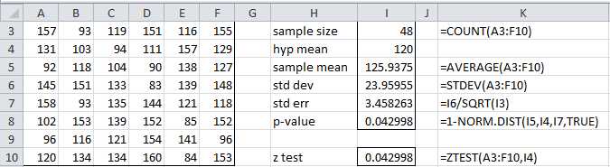
27. One sample testing of the mean

We first note that the average life of the motors in the sample is 125.9375, which is more than 120 months. But is this a statistically significant result or merely due to chance?  Keep in mind that even if the company’s claim is false any given sample may have a mean larger than 120 months.

Now let’s assume that the population of motors is distributed with mean μ and standard deviation σ. To perform the analysis we first define the null hypothesis as follows:

      H₀: μ < 120

The complement of the null hypothesis (called the alternative hypothesis) is therefore

      H₁: μ ≥ 120

Usually in an analysis we are actually testing the validity of the alternative hypothesis by testing whether or not to reject the null hypothesis. When performing such analyses, there is some chance that we will reach the wrong conclusion. There are two types of errors:

• Type I – H₀ is rejected even though it is true (false positive)
• Type II – H₀ is not rejected even though it is false (false negative)

The acceptable level of a Type I error (called the significance level) is designated by alpha (α), while the acceptable level of a Type II error is designated beta (β).

Typically, a significance level of α = .05 is used (although sometimes other levels such as α = .01 may be employed). This means that we are willing to tolerate up to 5% of type I errors, i.e. we are willing to accept the fact that in 1 out of every 20 samples we reject the null hypothesis even though it is true.

For our analysis we use the Central Limit Theorem. Since the sample size is sufficiently large we assume that the sample means have a normal distribution with mean μ and standard deviation σn, as depicted in Figure 28.

28. Right tailed critical region

Keep in mind that this curve represents the distribution of all possible values for the sample mean. We need to perform our test based on the observed sample mean of 125.9375.

The next step in the analysis is to determine the probability that the observed sample mean has a value of 125.9375 or higher under the assumption that the null hypothesis is true. If this probability is low (i.e. less than α) then we will have grounds for rejecting the null hypothesis; otherwise we would not reject the null hypothesis (also called retaining the null hypothesis).

Retaining the null hypothesis is not the same as positing that it is true. It merely means that based on the one observed sample we don’t have sufficient evidence for rejecting it.

The p-value (i.e. the probability value) is the value p of the statistic used to test the null hypothesis. If p < α then we reject the null hypothesis. For our problem the p-value is the probability that the observed sample mean has a value of 125.9375 or higher under the assumption that the null hypothesis is true. This is the same as testing whether the p-value falls in the shaded area of Figure 28 (i.e. the critical region), in what is called a one-tailed test.

The p-value for our example is calculated in cell I8 of Figure 28. Since p-value = .042998 < .05 = α, we see that the observed value does fall in the critical region and so we reject the null hypothesis, thereby showing that we have sufficient grounds for accepting the company’s claim that their motors last at least 120 months on average.

Note that the population standard deviation σ is unknown. For the analysis shown in Figure 28, we made the assumption that the sample standard deviation is a good estimate of the population standard deviation. For large enough samples this is a reasonable assumption, although it introduces additional error. In chapter 6 we show how to perform the same type of analysis using the t distribution without having to make this assumption.

To solve this problem we could also use Excel’s Z.TEST function (called ZTEST for versions of Excel prior to Excel 2010). See cell I10 in Figure 27.

Z.TEST(R, μ0, σ) = 1 – NORM.DIST(x, μ0, σ/n) where x = AVERAGE(R) = the sample mean of the data in range R and n = COUNT(R) = sample size. The third parameter is optional; when it is omitted the value of the sample standard deviation of R is used instead; i.e. Z.TEST(R, μ0) = Z.TEST(R, μ0, STDEV.S(R)).

We make one final observation. If we had tried to test the null hypothesis H₀: μ = 120, then the alternative hypothesis would become H₀: μ ≠ 120. In this case we would have two critical regions where we would reject the null hypothesis, as shown in Figure 29.

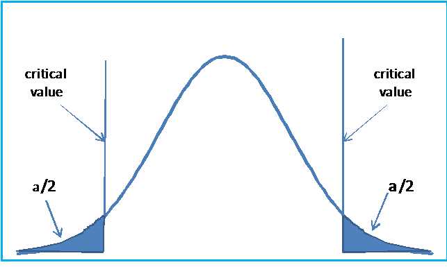
29. Two tailed hypothesis testing

This is called a two-tailed test, which is more commonly used than the one tailed test.