Linear Regression

---

Linear Regression Analysis

The goal of linear regression is to create a model from observed data which captures the relationship between an independent variable x and a dependent y and to use this model to predict the values of the dependent variable based on values of the independent variable (especially for values of the independent variable that were not originally observed). Even when we can make such predictions, this doesn’t imply that we can claim any causal relationship between the independent and dependent variables.

Regression Line

Essentially we are looking for a straight line that best fits the observed data x1,y1, …, xn,yn.

Recall that the equation for a straight line is y=bx+a, where

b = the slope of the line

a = y-intercept, i.e. the value of x where the line intersects with the y-axis

Using a technique called ordinary least squares, it turns out that

b=cov(x, y) / var(x)

a=y-bx

Excel provides the following functions where R1 is a range containing y data values and R2 is a range with x data values:       

SLOPE(R1, R2) = slope of the regression line as described previously

INTERCEPT(R1, R2) = y-intercept of the regression line as described previously

From our previous observation:         

b = SLOPE(R1, R2) = COVARIANCE.S(R1, R2) / VAR.S(R2)

a = INTERCEPT(R1, R2) = AVERAGE(R1) – b * AVERAGE(R2)

Example: Find the regression line for the data in Figure 66 (repeated on the left side of Figure 75). Based on this model what is the life expectancy of someone who smokes 10, 20 or 30 cigarettes a day?

The results are shown on the right side of Figure 75.

75. Regression line and predictions

The regression line is therefore

y = -0.6282x + 85.7204

For any value of x (= # of cigarettes smoked), the regression equation will generate a value for y which is a prediction of the life expectancy of a person who smokes that number of cigarettes.

For example, if a person smokes 30 cigarettes a day the model forecasts that the person will live to 66.87 years old (cell E10 in Figure 75).

Excel provides the following functions to help carry out these forecasts, where R1 is a range containing y data values and R2 is a range with x data values:

FORECAST(x, R1, R2) = calculates the predicted value y for the given value x of x.

TREND(R1, R2, R3) = array function which predicts the y values corresponding to the x values in R3.

We show how to use FORECAST in cell E9 of Figure 75 and TREND in cell E8 of Figure 75.

Actually TREND is an array function and so can be used to carry out multiple predictions. In fact if we highlight the range E8:E10, enter the formula =TREND(B4:B18,A4:A18,D4;D18) and then press Ctrl-Shift-Enter we will get the same results as shown in Figure 75.

Residuals

If R3 is omitted then TREND will generate the forecasted values of y for the various x values in R1. We can use this function to see how well the regression model predicts the y values which we have observed. This will help us determine how good the regression model really is. The result is shown in Figure 76.

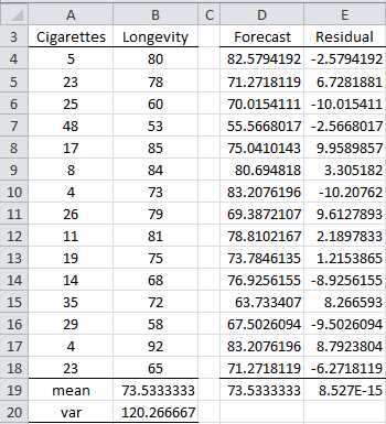
76. Residuals

Here we calculate the forecasted values in the range D4:D18 using the array formula

      =TREND(B4:B18,A4:A18)

The residuals, shown in the range E4:E18, are the differences between the actual y values and the forecasted y values. These are the error terms. They can be calculated by inserting the formula =B4-D4 in cell E4, highlighting the range E4:E18 and pressing Ctrl-D.

Although the forecasts are not 100% accurate, the mean of the forecasted values (cell D19) is the same as the mean of the observed values (cell B19) and the mean of the error terms (cell E19) is zero.

Model Fit

The sample variance of the observed y values (Longevity) can be calculated by the formula =VAR.S(B4:B18) and has a value 120.27. For our purpose we will call this variance the total mean square (abbreviated MST). As we have seen in chapter 3 the sample variance can be calculated by the formula

MST=i=1nyi-y2n-1=DEVSQ(B4:B18)COUNTB4:B18-1=1683.7314=120.27

The numerator is called the total sum of squares (abbreviated SST) and the denominator is the total degrees of freedom (abbreviated dfT). The only thing new is the terminology.

It turns out that we can segregate the value of SST (which represents the total variability of the observed y values) into the portion of variability explained by the model (the regression sum of squares SSReg) and the portion not explained by the model (the residual sum of squares SSRes) and similarly for the degrees of freedom. Thus we have:

SST=SSReg+SSRes

dfT=dfReg+dfRes

Now the values of each of these terms are:

SST=i=1nyi-y2          SSReg=i=1nyi-y2         SSRes=i=1nyi-y2

dfT=n-1          dfReg=k          dfRes=n-k-1

where the yi are the observed values for y and the yi are values of y predicted by the model and k = the number of independent variables in the model (k = 1 for now). We can also introduce mean squares values:

MST=SSTdfT          MSReg=SSRegdfReg          MSRes=SSResdfRes

Clearly the model fits the observed data well if SSRes is small in comparison to SSReg. Since SST =SSReg+ SSRes, this is equivalent to saying that SSRegSST is relatively close to 1.It turns out that this fraction is equal to the coefficient of determination, i.e. r2. It is common to use a capital R instead of a small r, and so we have

R2=SSRegSST

All these statistics can be calculated in Excel as shown in Figure 77.

77. Calculation of regression parameters in Excel

The formulas used are shown in Table 13 (based on the data Figure 76).

Table 13: Regression formulas

The residual mean squares term MSRes is a sort of variance for the error not captured by the model. The standard error of the estimate is simply the square root of MSRes. For current example this is the square root of 63.596 (cell J6 of Figure 77), i.e. 7.975. Excel provides the following function to calculate the standard error.

STEYX(R1, R2) = standard error of the estimate for the regression model where R1 is a range containing the observed y data values and R2 is a range containing the observed x data values.

Multiple Regression Analysis

We now extend the linear regression model introduced previously with one independent variable to the case where there are one or more independent variables.

If y is a dependent variable and x1,…,xk are independent variables, then the general multiple regression model provides a prediction of y from the xi of the form

y= β0+β1x1+β2x2+…+βkxk+ε

where β0,β1,…,βk are the regression coefficients of the model and ε is the random error. We further assume that for any given values of the xi the random error ε is normally and independently distributed with mean zero. Essentially the last of these conditions means that the model is a good fit for the data even if we eliminate the random error term.

Example: A jeweler prices diamonds on the basis of quality (with values from 0 to 8, with 8 being flawless and 0 containing numerous imperfections) and color (with values from 1 to 10, with 10 being pure white and 1 being yellow). Based on the price per carat of the 11 diamonds weighing between 1.0 and 1.5 carats shown in Figure 78, build a regression model which captures the relationship between quality, color and price.

Based on this model estimate the price for a diamond whose color is 4 and whose quality is 6.

78. Sample data

We use Excel’s Regression analysis tool by pressing Data > Analysis | Data Analysis and selecting Regression from the menu that is displayed. The dialog box shown in Figure 79 appears.

79. Dialog box for Regression data analysis

After filling in the fields as shown in the figure and pressing the OK button, the output shown in Figure 80 will be displayed.

The calculations of the values in Figure 80 are extensions of the approaches described earlier in this chapter for the case where there is only one independent variable (see especially Table 13). Adjusted R Square (cell B6) is an attempt to create a better estimate of the true value of the population coefficient of determination, and is calculated by the formula

      =1-(1-F7)*(F10-1)/(F10-F14-1)

The calculations of the regression coefficients (B17:B19) and the corresponding standard errors (C17:C19) use the method of least squares, but is beyond the scope of this book. The calculation of the p-values and confidence intervals for these coefficients is as described in chapter 7.

One of the key results of the analysis in Figure 80 is that the regression model is given by the formula

Price = 1.7514 + 4.8953 ∙ Color + 3.7584 ∙ Quality

80. Regression data analysis

Since the p-value (cell F12) = 0.00497 < .05, we reject the null hypothesis and conclude that the regression model is a good fit for the data.

Note that the Color and Quality coefficients are significant (p-value < .05), i.e. they are significantly different from zero, while the intercept coefficient is not significantly different from zero (p-value = .8077 > .05).

That R square = .8507 indicates that a good deal of the variability of price is captured by the model, which supports the case that the regression model is a good fit for the data.

If a diamond has color 4 and quality 6, then we can use the model to estimate the price as follows:

      Price = 1.75 + 4.90 ∙ Color + 3.76 ∙ Quality = 1.75 + 4.90 ∙ 4 + 3.76 ∙ 6 = 43.88305

We get the same result using the TREND function as shown in Figure 81.

81. Prediction using regression model