Distributions

Discrete Distributions

The (probability) frequency function f, also called the probability density function (abbreviated pdf), of a discrete random variable x is defined so that for any value t in the domain of the random variable:

ft=P(x=t)

where P(x=t) = the probability that x assumes the value t.

The corresponding (cumulative) distribution function Fx is defined by

Ft= u≤tf(u)

for any value t in the domain of the random variable x.

For any discrete random variable defined over the domain S with frequency function f and distribution function F

0 ≤ft≤1 for all t in S

t∈Sf(t)=1

Ft= P(x≤t)

Pt1<x≤t2=Ft2-F(t1)

A frequency function can be expressed as a table or a bar chart, as described in the following example.

Example: Find the distribution function for the frequency function given in columns A and B in Figure 22. Also show the graph of the frequency and distribution functions.

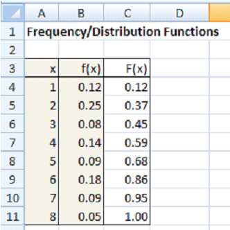
22. Table defining the frequency and distribution functions

Given the frequency function f(x) defined in the range B4:B11 of Figure 22, we can calculate the distribution function F(x), in the range C4:C11, by putting the formula =B4 in cell C4 and the formula =B5+C4 in cell C5 and then copying this formula into cells C6 to C11 (e.g., by highlighting the range C5:C11 and pressing Ctrl-D).

From the table in Figure 22, we can create the charts in Figure 23.

23. Charts of frequency and distribution functions

Continuous Distributions

While for a discrete random variable x, the probability that x assumes a value between a and b (exclusive) is given by a<x<bf(x), the frequency function f of a continuous random variable can assume an infinite number of values (even in a finite interval) and so we can’t simply sum up the values in the ordinary way. For continuous variables, the equivalent formulation is that the probability that x assumes a value between a and b is given by Area_a<x<b f(x), i.e. the area under the graph of y=f(x) bounded by the x-axis and the lines x=a and x=b.

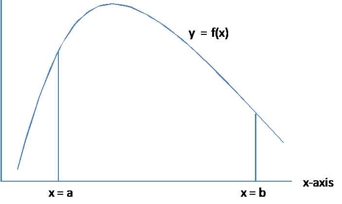
24. Area under the curve y=fx

For a continuous random variable x, f is a frequency function, also called the probability density function (pdf) provided:

f is the frequency function, more commonly called the probability density function for a particular random variable provided the area of the region indicated in Figure 24 represents the probability that x assumes a value between a and b inclusively. f only takes non-negative values and the area between the curve y=f(x) and the x-axis is 1.

The corresponding (cumulative) distribution function F is defined by

Fx= Areat<xft

For any continuous random variable with distribution function F

Fb= P(x<b)

F(b)-F(a)= P(a<x<b)

Note that the probability that x takes any particular value a is not f(a). In fact for any specific value a, the probability that x takes the value a is considered to be 0.

Essentially the area under a curve is a way of summing when dealing with an infinite range of values in a continuum. For those of you familiar with calculus, Areaa<x<bfx=abfxdx.

Excel Distribution Functions

The following table provides a summary of the various distribution functions provided by Excel. The entries labelled PDF/CDF specify the probability density function (where the last argument for the function is FALSE) as well as the (left tailed) cumulative distribution function (where the last argument of the function is TRUE.

Table 6: Excel Distribution Functions

The functions listed in Table 6 are not available for versions of Excel prior to Excel 2010. For earlier releases of Excel, a similar collection of functions is available, as summarized in Table 7 Here the column labelled PDF indicates whether the function in the CDF column (cumulative distribution function) also provides the probability density function (pdf) when the last argument in the function is FALSE (instead of TRUE).

Table 7: Distribution Functions for versions of Excel prior to Excel 2010