
Statistics Using Excel Succinctly®

CHAPTER 8
Chi-Square and F Distribution
Chi-Square Distribution
Basic Concepts
The chi-square distribution with k degrees of freedom has the probability density function
fx=xk2-1e-x22k2Γk2
where Γ is the gamma function and k does not have to be an integer and can be any positive real number. Note that chi-square is commonly written as χ2.
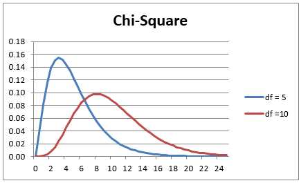
The following are the graphs of the probability density function with degrees of freedom df = 5 and 10. As df grows larger the fat part of the curve shifts to the right and becomes more like the graph of a normal distribution.
- Chart of the chi-square distribution
The key relationship between the chi-square and normal distribution is that if x has a standard normal distribution then x2 has a chi-square distribution with 1 degree of freedom.
Excel Functions
Excel provides the CHISQ.DIST, CHISQ.INV, CHISQ.DIST.RT and T.INV.RT functions to calculate values for the chi-square distribution and its inverse. These functions were not available prior to Excel 2007. The following table lists how these functions are used as well as
their equivalents using the functions CHIDIST and CHIINV, which were used prior to Excel 2010.
Table 9 – Formulas for the chi-square distribution in Excel
Tail | Distribution | Inverse |
|---|---|---|
Right tail | CHISQ.DIST.RT(x, df) = CHIDIST(x, df) | CHISQ.INV.RT(α, df) = CHIINV(α, df) |
Left tail | CHISQ.DIST(x, df, TRUE) =1- CHIDIST(x, df) | CHISQ.INV(α, df) = CHIINV(1-α, df) |
CHISQ.DIST has two forms: CHISQ.DIST(x, df, TRUE) is the value of the cumulative chi-square distribution function with df degrees of freedom at x, while CHISQ.DIST(x, df, FALSE) is the value of the probability density function at x.
Contingency Tables
The chi-square distribution is commonly used to determine whether two sets of data are independent of each other. Such data are organized in what are called contingency tables, as described in the following example.
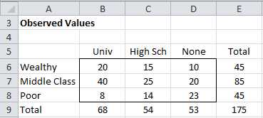
Example: A survey is conducted of 175 young adults whose parents are classified either as wealthy, middle class or poor, to determine their highest level of schooling (graduated from university, graduated from high school or neither). The results are summarized in the contingency table in Figure 44 (Observed Values). Based on the data collected is a person’s level of schooling independent of their parents’ wealth?
- Contingency Table (observed values)
We set the null hypothesis to be
H0: Highest level of schooling attained is independent of parents’ wealth
To use the chi-square test, we need to calculate the expected values that correspond to the observed values in the table in Figure 44. To accomplish this we use the fact that if two events are independent, then the probability that both events occur is equal to the product of the probabilities that each will occur.
We also assume that the proportions for the sample are good estimates of the probabilities of the expected values.
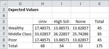
We now show how to construct the table of expected values (see Figure 45). We know that 45 of the 175 people in the sample are from wealthy families, and so the probability that someone in the sample is from a wealthy family is 45/175 = 25.7%. Similarly the probability that someone in the sample graduated from university is 68/175 = 38.9%. But based on the null hypothesis, the event of being from a wealthy family is independent of graduating from university, and so the expected probability of both is simply the product of the two events or 25.7% ∙ 38.9% = 10.0%, Thus, based on the null hypothesis, we expect that 10.0% of 175 = 17.5 people are from a wealthy family and have graduated from university.
- Expected Values
Thus, for example, cell H6 can be calculated by the formula =H$9*$K6/$K$9. If you highlight the range H6:J8 and press Ctrl-D and then Ctrl-R you will fill in the rest of the table.
Alternatively you can fill in the table of expected values by highlighting the range H6:J8 and entering the array formula
=MMULT(K6:K8,H9:J9)/K9
Independence Testing
The Pearson’s chi-square test statistic is defined as:
i=1kobsi-expi2expi
For sufficiently large samples, the Pearson’s chi-square test statistic has approximately a chi-square distribution with (row count – 1) (column count – 1) degrees of freedom.
The test requires that the following conditions be met:
- Random sample: Data must come from a random sampling of the population.
- Independence: The observations must be independent of each other. This means chi-square cannot be used to test correlated data (e.g., matched pairs).
- Cell size: All the expected frequency values in the contingency table are at least 5, although with large tables occasional values lower than 5 will probably still yield good results. With a 2 × 2 contingency table it is better to have even larger frequency values.
In Figure 46 we show how to use the chi-square test to carry out the analysis.
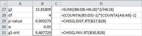
- Chi-square test
Since p-value = 0.003273 < .05 = α, we reject the null hypothesis and conclude that a person’s level of schooling is not independent of their parents’ wealth.
Excel provides the following function which carries out the chi-square test for independence for contingency tables.
CHISQ.TEST(R1, R2) = CHISQ.DIST.RT(x, df) where x is the chi-square statistic, R1 = the array of observed data, R2 = the array of expected value and df = (row count – 1) (column count – 1).
For our example, CHISQ.TEST(B6:D8,H6:J8) = 0.003273.
The CHISQ.TEST function is only available in versions of Excel starting with Excel 2010. For previous versions of Excel the equivalent function CHITEST can be used.
F Distribution
Basic Concepts
If x1 and x2 have chi-square distributions with df1 and df2 degrees of freedom respectively, then the quotient F = x1 /x2 has F distribution with df1, df2 degrees of freedom.
The F distribution is commonly used to compare two variances, and is useful in ANOVA, regression and other commonly used tests. In particular if we draw two independent samples of size n1 and n2 respectively from two different normal populations with the same variance then the quotient of the two sample variances has F distribution with n1-1,n2-1 degrees of freedom.
Excel Functions
Excel provides the F.DIST, F.INV, F.DIST.RT and F.INV.RT functions to calculate values for the F distribution and its inverse. These functions were not available prior to Excel 2007. The following table lists how these functions are used as well as their equivalents using the functions FDIST and FINV which were available prior to Excel 2010.
Table 10: F distribution formulas in Excel
Tail | Distribution | Inverse |
|---|---|---|
Right tail | F.DIST.RT(x, df1, df2) = FDIST(x, df1, df2) | F.INV.RT(α, df1, df2) = FINV(α, df1, df2) |
Left tail | F.DIST(x, df1, df2, TRUE) = 1 – FDIST(x, df1, df2) | F.INV(α, df1, df2) = FINV(1-α, df1, df2) |
F.DIST has two forms: F.DIST(x, df, TRUE) is the value of the cumulative F distribution function with df degrees of freedom at x, while F.DIST(x, df, FALSE) is the value of the probability density function at x.
Hypothesis Testing
As we observed previously, if we draw two independent samples of size n1 and n2 respectively from two different normal populations with the same variance then the quotient of the two sample variances has F distribution with n1-1,n2-1 degrees of freedom.
This fact can be used to test whether the variances of two populations are equal. In order to deal exclusively with the right tail of the distribution, when taking ratios of sample variances we should put the larger variance in the numerator of the quotient.
In order to use this test, the following must hold:
- Both populations are normally distributed
- Both samples are drawn independently from each other.
- Within each sample, the observations are sampled randomly and independently of each other.
Example
A company is comparing two methods for producing high precision bolts and wants to choose the method with the least variability. It has taken a sample of the lengths of the bolts using both methods as given in the table on the left side of Figure 47.
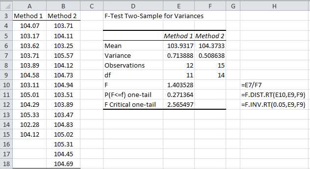
- F test to compare two variances
To carry out the test we use Excel’s F-Test Two Sample For Variances data analysis tool, which, as usual, can be accessed by selecting Data > Analysis|Data Analysis. The result is shown on the right side of Figure 47.
Since p-value = .271364 > .05 = alpha, we cannot reject the null hypothesis, and so conclude that there is no significant difference between the two variances.
Excel Test Function
Excel provides the following test statistic function.
F.TEST(R1, R2) = two-tailed F-test comparing the variances of the samples in ranges R1 and R2 = the two-tailed probability that the variance of the data in ranges R1 and R2 are not significantly different.
Note that unlike the F-Test data analysis tool or F.DIST, F.DIST.RT, F.INV and F.INV.RT functions, which are one-tailed, the F.TEST function is two-tailed. For the previously example
F.TEST(A4:A18,B4:B18) = .5427
which is double the value obtained for the one-tailed p-value in cell E11 of Figure 47.
- 1800+ high-performance UI components.
- Includes popular controls such as Grid, Chart, Scheduler, and more.
- 24x5 unlimited support by developers.