
Statistics Using Excel Succinctly®

CHAPTER 9
Analysis of Variance
Introduction
Essentially ANOVA is an extension of two sample hypothesis testing for comparing means (when variances are unknown) to more than two samples.
We start with the one factor case. We will define the concept of factor later, but for now we simply view this type of analysis as an extension of the two independent sample t test with equal population variances.
One-way ANOVA
One-way ANOVA Example
A food company wants to determine whether any of three new formulas for peanut butter is significantly tastier than their old formula. They create four random samples of ten people each, one for each type of peanut butter, and asked the people in the each sample to taste the peanut butter for that sample. They then asked all forty people to fill out a questionnaire rating the tastiness of the peanut butter they tried.
Based on the data in Figure 48, determine whether there is a significant difference between the four types of peanut butter.
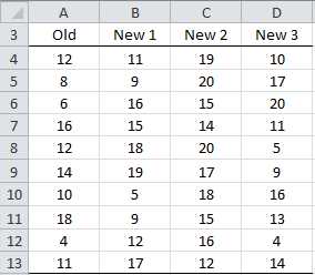
- Sample data
The null hypothesis for this example is that any difference between the four types of peanut butter is due to chance, i.e.
H0: μ1=μ2=μ3=μ4
Basic Concepts
Before we proceed with the analysis for this example, we review a few basic concepts.
Suppose we have k samples, which we will call groups (or treatments); these are the columns in our analysis (corresponding to the four types of peanut butter in the example). We will use the index j for these. Each group consists of a sample of size nj. The sample elements are the rows in the analysis. We will use the index i for these.
Suppose the jth group sample is {x1j,…, xnjj}, and so the total sample consists of all the elements {xij:1 ≤i ≤nj, 1 ≤j ≤k}. We will use the abbreviation xj for the mean of the jth group sample (called the group mean) and x for the mean of the total sample (called the total or grand mean).
Let the sum of squares for the jth group be SSj= ixij-xj2. We now define the following terms:
SST=jixij-x2
SSB=jnjxj-x2
SSW=jSSj=jixij-xj2
SST is the sum of squares for the total sample, i.e. the sum of the squared deviations from the grand mean. SSW is the sum of squares within the groups, i.e. the sum of the squared means across all groups. SSB is the sum of the squares between group sample means, i.e. the weighted sum of the squared deviations of the group means from the grand mean.
We also define the following degrees of freedom, where n= j=1knj:
dfT=n-1 dfB=k-1 dfW=j=1knj-1=n-k
Finally we define the mean square, as MS=SS/df, and so
MST=SST / dfT MSB=SSB / dfB MSW=SSW / dfW
We summarize these terms in the following table.
Table 11: Summary of ANOVA terms
df | SS | MS | |
|---|---|---|---|
n –1 | jixij-x2 | ||
k –1 | jnjxj-x2 | ||
n –k | jixij-xj2 |
Clearly MST is the variance for the total sample, MSW is the sum of the group sample variances and MSB is the variance for the “between sample” i.e. the variance of {n1x1, …, nkxk}.
It is also not hard to show that
SST=SSW+SSB
dfT=dfW+dfB
It turns out that if the null hypothesis is true, then MSW and MSB are both measures of the same error. Thus the null hypothesis becomes equivalent to the hypothesis that the population versions of these statistics are equal, i.e.
σB= σW
We can therefore use the F-test described in chapter 8 to determine whether or not to reject the null hypothesis. This means that if the xij are independently and normally distributed and all the μj are equal (null hypothesis) and all the σj2 are equal (homogeneity of variances), then the test statistic
F=MSBMSW
has an F distribution with dfB,dfW degrees of freedom.
Analysis
To carry out the analysis for the example, we will use the Anova: Single Factor data analysis tool. To access this tool, as usual, press Data > Analysis|Data Analysis and fill in the dialog box that appears as in Figure 49.
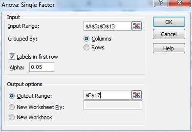
- Dialog box for Anova: Single factor data analysis tool
The output is as shown in Figure 50.

- Anova: Single factor data analysis
All the fields in Figure 50 are calculated as described previously. We see that the test statistics is F = 3.206928. Since p-value = F.DIST(3.206928, 3, 36) = 0.034463 < .05 = α, we reject the null hypothesis that there is no significant difference between the evaluations of the four different types of peanut butter.
Follow-up Analysis
Although we now know that there is a significant difference between the four types of peanut butter, we still don’t know where the differences lie.
It appears from Figure 50 that New 2 has a higher rating than the other types of peanut butter. We can use a t test to determine whether there is a significant difference between the rating for New 2 and the next highest rated peanut butter, New 1. The result is shown in Figure 51.
t-Test: Two-Sample Assuming Unequal Variances | ||
| New 1 | New 2 |
Mean | 13.1 | 16.6 |
Variance | 21.21111 | 7.155556 |
Observations | 10 | 10 |
Hypothesized Mean Difference | 0 | |
df | 14 | |
t Stat | -2.07809 | |
P(T<=t) one-tail | 0.028289 | |
t Critical one-tail | 1.76131 | |
P(T<=t) two-tail | 0.056577 | |
t Critical two-tail | 2.144787 |
|
- Follow-up analysis: New 1 vs. New 2
From Figure 51 we see that there is no significant difference between the two types of peanut butter based on a two-tailed test (0.056577 > .05). If we instead compare the New 2 with the Old formula we get the results shown in Figure 52.
t-Test: Two-Sample Assuming Unequal Variances | ||
| Old | New 2 |
Mean | 11.1 | 16.6 |
Variance | 18.76667 | 7.155556 |
Observations | 10 | 10 |
Hypothesized Mean Difference | 0 | |
df | 15 | |
t Stat | -3.41607 | |
P(T<=t) one-tail | 0.001915 | |
t Critical one-tail | 1.75305 | |
P(T<=t) two-tail | 0.003829 | |
t Critical two-tail | 2.13145 |
|
- Follow-up analysis: analysis: Old vs. New 2
This time we see that there is a significant difference between the two types of peanut butter, using a two-tailed t-test (.003829 < .05).
The problem with this approach is that doing multiple tests incurs higher amounts of what is called experimentwise error. Remember that when we use a significance level of α = .05, we accept that 5% of the time we will get a type I error. If we perform three such tests then we will essentially increase our overall type I error to 1 – (1 – .05)3 = .14. This means that 14% of the time we will have a type I error, which is higher than we would like.
The general approach for addressing this issue is to either reduce α using Bonferroni’s correction (e.g., for three tests we use α/3 = .05/3 = .0167) or to use a different type of test (e.g., Tukey’s HSD or REGWQ), which is beyond the scope of this book.
Levene’s Test
As mentioned previously, the ANOVA test requires that the group variances be equal. There is a lot of leeway here and even when the variance of one group is four times another, the analysis will be pretty good. Another option for testing homogeneity of group variances is Levene’s test.
For Levene’s test, the residuals eij of the group means from the cell means are calculated as follows:
eij=xij-xj
An ANOVA is then conducted on the absolute value of the residuals. If the group variances are equal, then the average size of the residual should be the same across all groups.
There are three versions of the test: using the mean (as described) or using the median or trimmed mean.
Example: Use Levene’s test (residuals from the median) to determine whether the 4 groups in the ANOVA example have significantly different population variances.
We begin by calculating the medians for each group (range B14:E14). E.g., cell B14 contains the formula =MEDIAN(B4:B13).
We next create the table (in range B19:E29) with the absolute residuals from the median. We do this by entering the formula =ABS(B4-B$14) in cell B20, highlighting the range B20:E29 and then pressing Ctrl-R followed by Ctrl-D.
Finally we use the Anova: Single Factor data analysis tool as described earlier in this chapter on the Input Range B19:E29. The output is shown on the right side of Figure 53.

- Levene’s test
Since p-value = .25752 > .05 = α, we cannot reject the null hypothesis, and so we conclude there is no significant difference between the 4 group variances. Thus the ANOVA test conducted previously satisfies the homogenity of variances assumption.
Factorial ANOVA
Example
A new fertilizer has been developed to increase the yield on crops, and the makers of the fertilizer want to better understand which of the three formulations (blends) of this fertilizer are most effective for wheat, corn, soy beans and rice (crops). They test each of the three blends on five samples of each of the four types of crops. The crop yields for the 5 samples of each of the 12 combinations are as shown in Figure 54.
Determine whether there is a difference between crop yields based on these three types of fertilizer.
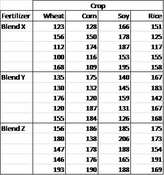
- Sample data for two factor ANOVA
Before we proceed with the analysis for this example, we review a few basic concepts.
Basic Concepts
We now extend the one factor ANOVA model described previously to a model with more than one factor.
A factor is an independent variable. A k factor ANOVA addresses k factors. The model for the last example contains two factors: crops and blends.
A level is some aspect of a factor; these are what we called groups or treatments in the one factor analysis described previously. The blend factor contains 3 levels and the crop factor contains 4 levels.
Let’s look at the two factor model in more detail.
Suppose we have two factors A and B where factor A has r levels and factor B has c levels. We organize the levels for factor A as rows and the levels for factor B as columns. We use the index i for the rows (i.e. factor A) and the index j for the columns (i.e. factor B).
This yields an r × c table whose entries are Xij: 1≤i≤r, 1≤j≤c, where Xij is a sample for level i of factor A and level j of factor B. Here Xij=xijk: 1≤k≤nij. We further assume that the nij are all equal of size m and use k as an index to the sample entries.
We use terms such as xi (or xi.) as an abbreviation for the mean of xijk: 1≤j≤r, 1≤k≤m. We use terms such as xj (or x.j) as an abbreviation for the mean of xijk: 1≤i≤c, 1≤k≤m.
We also expand the definitions of sum of squares, mean square and degrees of freedom for the one factor model described earlier to the two factor model as described in Table 12.
Table 12: Two factor ANOVA terminology
SS | df | MS |
|---|---|---|
Note that in addition to the A and B factors, the model also contains the intersection between these factors, labeled AB in the table, which consists of the m elements in each of the r × c combinations of factor levels.
It is not hard to show that
SST=SSA+SSB+SSAB+SSE
dfT=dfA+dfB+dfAB+dfE
It turns out that if the null hypothesis is true, then MSW and MSB are both measures of the same error. Thus the null hypothesis is equivalent to the hypothesis that the population versions of these statistics are equal, i.e.
σB= σW
We can therefore use the F-test described in chapter 8 to determine whether or not to reject the null hypothesis, i.e. if the xij are independently and normally distributed and all μj are equal (the null hypothesis) and all the σj2 are equal (homogeneity of variances), then the test statistic
F=MSBMSW
has an F distribution with dfB,dfW degrees of freedom.
Analysis
To carry out the analysis for the last example, we will use the Anova: Two Factor with Replication data analysis tool. To access this tool, as usual press Data > Analysis|Data Analysis and fill in the dialog box that appears as in Figure 55.
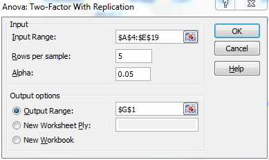
- Dialog box for Anova: Two-Factor with Replication analysis tool
After pressing the OK button the output shown in Figures 56 and 57 appear.
Anova: Two-Factor With Replication | |||||
SUMMARY | Wheat | Corn | Soy | Rice | Total |
Blend X |
|
|
|
|
|
Count | 5 | 5 | 5 | 5 | 20 |
Sum | 659 | 677 | 879 | 706 | 2921 |
Average | 131.8 | 135.4 | 175.8 | 141.2 | 146.05 |
Variance | 844.2 | 707.8 | 278.7 | 354.2 | 782.3658 |
Blend Y |
|
|
|
|
|
Count | 5 | 5 | 5 | 5 | 20 |
Sum | 716 | 798 | 701 | 827 | 3042 |
Average | 143.2 | 159.6 | 140.2 | 165.4 | 152.1 |
Variance | 498.7 | 978.3 | 165.7 | 217.3 | 511.0421 |
Blend Z |
|
|
|
|
|
Count | 5 | 5 | 5 | 5 | 20 |
Sum | 822 | 868 | 932 | 862 | 3484 |
Average | 164.4 | 173.6 | 186.4 | 172.4 | 174.2 |
Variance | 443.3 | 428.8 | 212.3 | 175.8 | 330.6947 |
Total |
|
|
|
| |
Count | 15 | 15 | 15 | 15 | |
Sum | 2197 | 2343 | 2512 | 2395 | |
Average | 146.4667 | 156.2 | 167.4667 | 159.6667 | |
Variance | 705.8381 | 871.0286 | 605.981 | 404.9524 | |
- Two-Factor ANOVA descriptive statistics
ANOVA | ||||||
Source of Variation | SS | df | MS | F | P-value | F crit |
Sample | 8782.9 | 2 | 4391.45 | 9.933347 | 0.000245 | 3.190727 |
Columns | 3411.65 | 3 | 1137.217 | 2.572355 | 0.064944 | 2.798061 |
Interaction | 6225.9 | 6 | 1037.65 | 2.347138 | 0.045555 | 2.294601 |
Within | 21220.4 | 48 | 442.0917 | |||
Total | 39640.85 | 59 |
|
|
|
|
- Two-Factor ANOVA
We now draw some conclusions from the ANOVA table in Figure 57. Since the p-value (crops) = .0649 > .05 = α, we can’t reject the Factor A null hypothesis, and so conclude (with 95% confidence) that there are no significant differences between the effectiveness of the fertilizer for the different crops.
Since the p-value (blends) = .00025 < .05 = α, we reject the Factor B null hypothesis, and conclude that there is a statistical difference between the blends.
We also see that the p-value (interactions) = .0456 < .05 = α, and so conclude there are significant differences in the interaction between crop and blend. We can look more carefully at the interactions by plotting the mean interactions between the levels of the two factors (see Figure 58). Lines that are roughly parallel indicate the lack of interaction, while lines that are not roughly parallel indicate interaction.
From the first chart we can see that Brand X has quite a different pattern from the other brands (especially regarding Soy). Although less dramatic, Brand Y is also different from Brand Z (especially since the line for Brand Y is trending up towards Soy, but trending down towards Rice, exactly the opposite of Brand Z).
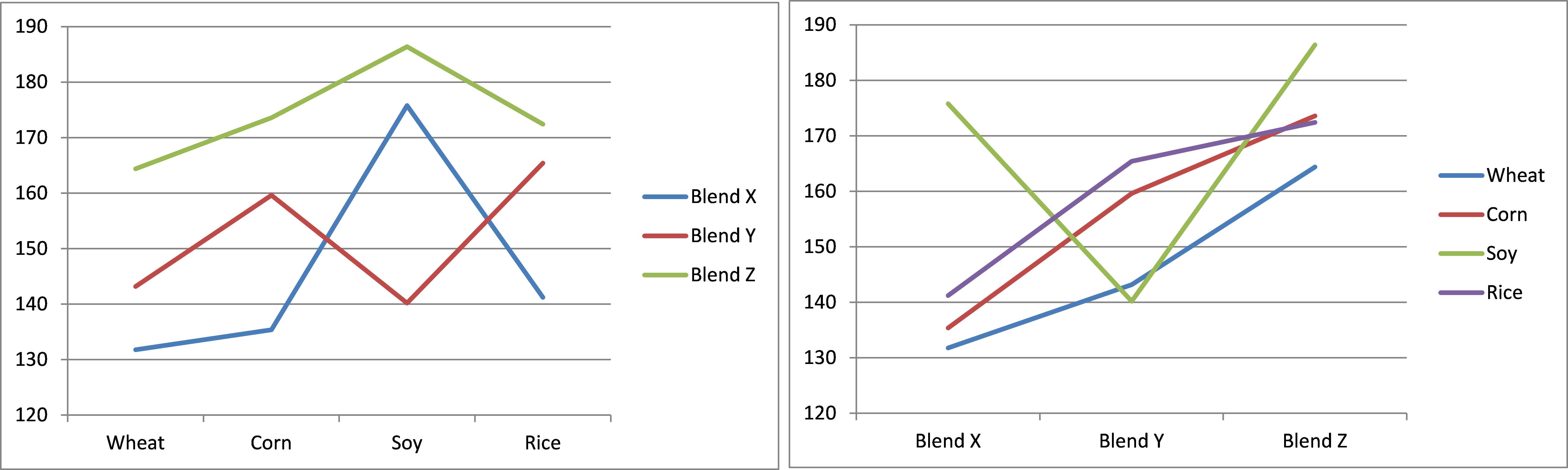
- Interaction plots
Follow-up tests are carried out as for one-way ANOVA, although there are more possibilities.
ANOVA with Repeated Measures
Basic Concepts
ANOVA with repeated measures is an extension of the t test with paired samples test to more than two variables. As for the paired samples t test, the key difference between this type of ANOVA and the tests we have considered until now is that the variables under consideration are not independent.
Some examples of this type analysis are:
- A study is made of 30 subjects each of whom is asked to take a test on driving a car, a boat and an airplane.
- A study is made of 30 rats, each of whom is given training once a day for 10 days with their scores recorded each day
- A study is made of 30 married couples and the husband’s IQ is compared with his wife’s
The important characteristic of each of these examples is that the treatments are not independent of each other. The most common of these analyses is to compare the results of some treatment given to the same participant over a period of time (like the second example).
Example
A program has been developed to reduce the levels of anxiety for new mothers. In order to determine whether the program is successful a sample of 15 women was selected and their level of anxiety was measured (low scores indicate higher levels of anxiety) before the program, as well as 1, 2 and 3 weeks after the beginning of the program. Based on the data in range G5:K20 of Figure 59, determine whether the program is effective in reducing anxiety.
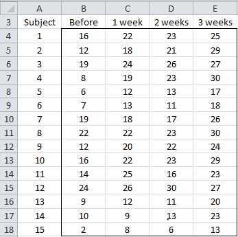
- Sample data
Analysis
To perform ANOVA with repeated measures we use Excel’s Anova: Two Factor without Replication data analysis tool.
To access this tool, press Data > Analysis|Data Analysis and fill in the dialog box that appears as in Figure 60.

- Dialog box for Anova: Two-Factor without Replication
After pressing the OK button the output shown in Figures 61 and 62 appear.
Anova: Two-Factor Without Replication | ||||
SUMMARY | Count | Sum | Average | Variance |
1 | 4 | 86 | 21.5 | 15 |
2 | 4 | 80 | 20 | 50 |
3 | 4 | 96 | 24 | 12.66667 |
4 | 4 | 80 | 20 | 84.66667 |
5 | 4 | 48 | 12 | 20.66667 |
6 | 4 | 49 | 12.25 | 20.91667 |
7 | 4 | 80 | 20 | 16.66667 |
8 | 4 | 97 | 24.25 | 14.91667 |
9 | 4 | 78 | 19.5 | 27.66667 |
10 | 4 | 90 | 22.5 | 28.33333 |
11 | 4 | 78 | 19.5 | 28.33333 |
12 | 4 | 107 | 26.75 | 6.25 |
13 | 4 | 52 | 13 | 23.33333 |
14 | 4 | 55 | 13.75 | 40.91667 |
15 | 4 | 29 | 7.25 | 20.91667 |
Before | 15 | 196 | 13.06667 | 39.35238 |
1 week | 15 | 270 | 18 | 34.28571 |
2 weeks | 15 | 278 | 18.53333 | 44.69524 |
3 weeks | 15 | 361 | 24.06667 | 26.35238 |
- ANOVA descriptive statistics
ANOVA | ||||||
Source of Variation | SS | df | MS | F | P-value | F crit |
Rows | 1702.833 | 14 | 121.631 | 15.82722 | 1.95E-12 | 1.935009 |
Columns | 910.9833 | 3 | 303.6611 | 39.51389 | 2.69E-12 | 2.827049 |
Error | 322.7667 | 42 | 7.684921 | |||
Total | 2936.583 | 59 |
|
|
|
|
- Two-Factor ANOVA with Repeated Measures
For ANOVA with repeated measures we aren’t interested in the analysis of the rows, only the columns, which correspond to variations by time. Since the test statistic F = 29.13 > 2.83 = F-crit (or p-value = 2.69E-12 < .05 = α) in Figure 62, we reject the null hypothesis, and conclude there are significant differences between the means.
Assumptions
The requirements for ANOVA with matched samples are as follows:
- Subjects are independent and randomly selected from the population.
- Normality (or at least symmetry) – although overly restrictive it is sufficient for this condition to be met for each treatment (i.e. for each column in the data range).
- Sphericity
Data satisfies the sphericity property when the pairwise differences in variance between the samples are all equal. This assumption is stronger than the homogeneity assumption for the other versions of ANOVA described previously.
We perform the test for sphericity in Figure 63.
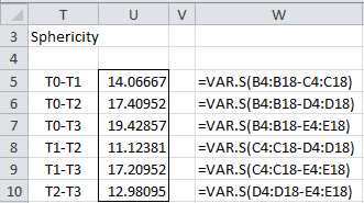
- Sphericity
Although the values in column U of Figure 63 are not equal they aren’t too far apart, and especially since the p-value obtained in Figure 62 is so low, we don’t expect sphericity to be much of a problem for this example.
When sphericity is a problem, we can use a variety of correction factors to improve the ANOVA results. Unfortunately, explaining this will take us too far afield for our purposes here. If you would like more information, please consult www.real-statistics.com.
Follow-up Analysis
Since the mean score of 24.07 in week 3 is much higher than the mean Before score of 13.07 (see Figure 61), it appears there is a positive effect from taking the program. We can confirm this by using a paired sample t test comparing Before with 3 weeks, as shown in Figure 64.
t-Test: Paired Two Sample for Means | ||
| Before | 3 weeks |
Mean | 13.06667 | 24.06667 |
Variance | 39.35238 | 26.35238 |
Observations | 15 | 15 |
Pearson Correlation | 0.718509 | |
Hypothesized Mean Difference | 0 | |
df | 14 | |
t Stat | -9.66536 | |
P(T<=t) one-tail | 7.11E-08 | |
t Critical one-tail | 1.76131 | |
P(T<=t) two-tail | 1.42E-07 | |
t Critical two-tail | 2.144787 |
|
- Paired t test: Before vs. 3 weeks
We see that p-value = 1.42E-07, which is considerably less than .05, thus confirming that there is a significant difference between Before and 3 weeks after.
In fact we can see from Figure 65 that there is a significant improvement in the scores even after 1 week.
t-Test: Paired Two Sample for Means | ||
| Before | 1 week |
Mean | 13.06667 | 18 |
Variance | 39.35238 | 34.28571 |
Observations | 15 | 15 |
Pearson Correlation | 0.810897 | |
Hypothesized Mean Difference | 0 | |
df | 14 | |
t Stat | -5.09437 | |
P(T<=t) one-tail | 8.17E-05 | |
t Critical one-tail | 1.76131 | |
P(T<=t) two-tail | 0.000163 | |
t Critical two-tail | 2.144787 |
|
- Paired t test: before vs. 1 week
In fact even if we apply Bonferroni’s correction factor using .05/2 = .025 (because we have now performed two t tests), we see that p-value = .000163 < .025), confirming that there is a significant improvement after only one week.
- 1800+ high-performance UI components.
- Includes popular controls such as Grid, Chart, Scheduler, and more.
- 24x5 unlimited support by developers.