T-Tests

Hypothesis test when population parameters are unknown

In this chapter, you’ll determine if a sample mean is significantly different from a particular value (which we'll call m₀) or another sample when we don’t know population parameters. To do this, we’ll use the same concept as in Chapter 5: determine how many standard errors are separating from m₀ or and the mean of the other sample. The procedure is exactly the same—only the calculation of standard error changes.

If we have a sample but don’t know population parameters, we have to make conjectures about the population based on s (sample standard deviation) and (mean).

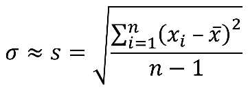
We use the sample standard deviation, s, to approximate the population standard deviation, σ. (Remember, we divide the sum of squares by n-1 rather than n in order to make the result slightly bigger and therefore to better approximate s.)

Consequently, we're also approximating the standard error: s / Ön. Because we use s to approximate the standard error, we will have more error and therefore we will use a different kind of distribution that has thicker tails: the t-distribution.

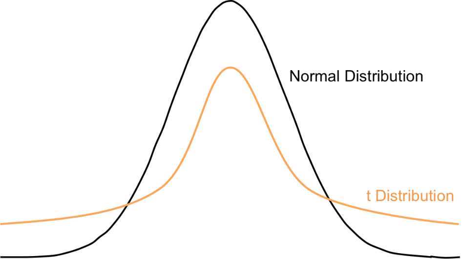
Figure 34: The t-distribution has fatter tails to compensate for the greater error involved in calculating the standard error, which uses s to approximate s.

Because we’re using an entirely different distribution that accounts for greater error, these statistical tests are called t-tests.

Again, we integrate the PDF of the t-distribution to calculate probabilities. And also again, we have a table (this time the t-table) that provides the probabilities for us. A few things differ between this table and the z-table:

• The t-table asks for the degrees of freedom, which is equal to n – 1.
• The body of the t-table gives t-critical values rather than probabilities (which are the column headers).
• The t-table provides t-critical values for both one-tailed and two-tailed tests.

Tip: More detail on degrees of freedom can be found in Street-Smart Stats, Chapter 10.

The t-table supplies t-critical values because we no longer care about probabilities under this curve the way we do with standard distributions. We only care about whether or not our sample mean falls within the critical region, and to learn this we simply need to compare the distance in terms of standard errors (i.e. the t-statistic) with the t-critical value marking our chosen alpha level.

We denote the t-critical value t_{(α, df)} to specify the alpha level we’re using and the degrees of freedom. Here is the t-statistic:

If we perform a two-tailed test (high or low tails) at a = 0.05, and our sample size is n = 37, then t_{(0.05, 36)} = 2.021 (with degrees of freedom rounded from 36 to 40). Therefore, if the t-statistic is either less than -2.021 or greater than 2.021, t falls in the critical region and our results are significant.

We’ll cover two types of t-tests in this chapter:

1. One-sample t-tests in which we compare a sample to a constant, denoted m_0.
2. Two-sample t-tests in which we compare two samples with each other.

One-sample t-tests

We perform a one-sample t-test when we want to know if our sample and a particular value (m₀) are likely to belong to the same population. In other words, if m₀ were a sample mean, would it likely be in the same sampling distribution as ?

A t-test answers this question by estimating the standard error and then determining the number of standard errors that separate and m₀. We use the t-table to determine if the probability of those errors being this distance apart is less than our alpha level.

In this case, our t-statistic is

with null and alternative hypotheses:

Note that m₀ is a constant.

Example

A major technology company has just released a new product. The business development team has decided that on a scale of 1 to 10 (10 being highest satisfaction), their goal is for customer satisfaction to achieve more than 8. The R&D department decides to perform a one-sample t-test to determine if customer satisfaction so far is significantly more than 8. They send out a survey to a random sample of 50 customers who bought the product, and they find the average satisfaction score is 8.7 with sample standard deviation 1.6. Does it appear that most people will rate their satisfaction above 8?

In this case, we’ll do a one-sample t-test because we want to determine if the customer satisfaction score is greater than 8 rather than simply different from 8. Therefore, our null and alternative hypotheses are:

H₀: m_S = 8
H_a: m_S > 8

Now, we must compare this t-statistic with the t-critical value, t_{(0.05, 49)}. The t-table tells us that for a one-tailed test, t_{(0.05, 40)} = 1.684. (Note that t_{(0.05, 60)} = 1.671, so for our particular sample with df = 49, t_{(0.05, 49)} will fall between 1.671 and 1.684.) Because the t-statistic is greater than the t-critical value, our results are significant, and we can say that customer satisfaction is statistically significantly greater than 8 and we reject the null. (Recall that the null hypothesis states that the results are not significant, so rejecting the null means we’ve concluded that there is a significant difference between the observed customer satisfaction and the goal of 8.)

Let’s do a one-sample t-test in R for the variable “income2011” of our NCES data.

Code Listing 8

This t-test takes mean(income2011)–40,000, so if the t-statistic is negative, mean(income2011) is less than 40,000. You should find that t = -47, indicating that the true population mean is a lot less.

You've just learned how to compare a sample to a particular value, m₀. We also use t-tests to determine if two samples are significantly different and therefore most likely come from two different populations. In this case, we would do a two-sample t-test.

Two-sample t-tests

There are two types of two-sample t-tests: dependent-samples t-tests and independent-samples t-tests. We use dependent samples when measurements are taken from the same subjects. For example, we might use a dependent-samples t-test to determine if there is a significant difference between:

• Children’s heights at age 8 and age 10.
• Students’ scores on a pre-assessment and post-assessment for a course.
• The effectiveness of two different sleeping pills on the same people.

This method controls for individual differences, in effect holding them constant to determine if any difference is most likely due to the intervention (in the examples above, the interventions are age, course materials, and the sleeping pill).

We use independent samples when subjects differ between the two groups. For example, we might use this test to determine if a significant difference exists between:

• Different countries’ carbon emissions.
• Men’s and women’s wages.
• Flight costs in January vs. August.

Independent samples no longer have the benefit of holding individual subjects constant. In order to determine if there is a significant difference between groups, samples need to be random.

To help us think about each two-sample test, let's assign symbols representing each sample's statistics.

Sample 1
Mean = ₁
Sample standard deviation = s₁

Sample 2
Mean = ₂
Sample standard deviation = s₂

Our null and alternative hypotheses are:

We can rewrite them as:

Here the difference between the two populations is significantly less than, greater than, or different from 0.

Dependent samples t-test

The dependent-samples t-test is almost exactly like the one-sample t-test. The only thing that changes is that we take the difference between each value measured from each subject, and that group of differences becomes our sample. We then test to see if this difference is significantly different than 0.

Example

Let’s say we want to determine whether an online course was effective in improving students’ abilities. To measure this, students were given a standard test before they went through the course, and they took a similar test after completing the course

Our data looks something like this:

The differences (which we’ll denote as d_i) become our sample. Now we’ll proceed as we would for a one-sample t-test, with m₀ = 0.

Let’s say that upon taking each difference d_i, we find the following mean and sample standard deviation:

_i = 4.2
s_i = 3.1

We can now find our t-statistic:

This is much greater than the t-critical value t_{(0.05, 33)} » 2.042 for a two-tailed test. Therefore, we reject the null and conclude that the online course improved scores.

Now we’ll perform a dependent-samples t-test in R. This time we won’t use the NCES data because there isn’t necessarily anything we would want to perform a t-test on, so we’ll use a different data set. Let’s say we want to know whether stocks significantly dropped following the Greek bank closures on June 29, 2015, so we analyze the previous closing price (on June 28) and the closing price on June 29 for 15 companies.

First, visit turnthewheel.org/street-smart-stats/afterward and click “Stock data set” (the second link under “Resources”) to view the data in a Google spreadsheet. Download the data as a .csv, rename it “stocks.csv,” and save the file to your working directory. The code follows.

Code Listing 9

The t.test() function returns a t-statistic for the first argument minus the second argument. In other words, if the t-statistic is negative, that means the first argument is less than the second. To ensure you’re doing a dependent-samples t-test, type paired=TRUE.

In this example, we see that t = -6.4302, which is statistically significant—i.e. the average stock price dropped more than $1 between yesterday and today.

Note: This example has been simplified for the purpose of explaining how to apply a t-test. However, a robust t-test must use a larger sample size or normally distributed data. Otherwise, comparing two data sets doesn’t make much sense because there will be too much error and uncertainty in the way they are distributed (i.e. a $1 drop in price may mean something completely different for one stock versus another).

Independent-samples t-test

Things get a bit more complicated with independent-sample t-tests because we can’t simply subtract the values as we can with a dependent-sample test. Not only do we have different sample sizes, but we also have to account for the standard deviations of both samples rather than simply taking the standard deviation of the differences.

We can think about whether or not two samples are significantly different (i.e. they could come from the same population) in the context of confidence intervals. We can use each sample to determine a range in which we're pretty sure each population mean lies:

If these intervals overlap a lot, the two samples might have been taken from the same population, and it’s due to error that the samples are different (because every sample taken from a population will most likely include different values than the next). However, we also have to consider the standard deviation of each population distribution. The greater the standard deviation of each distribution, the more likely the distributions will overlap. And the more they overlap, the more likely the two samples came from the same population.

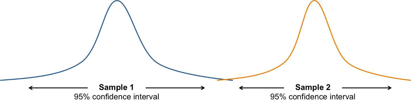
Figure 35: Most likely, these samples come from two different populations.

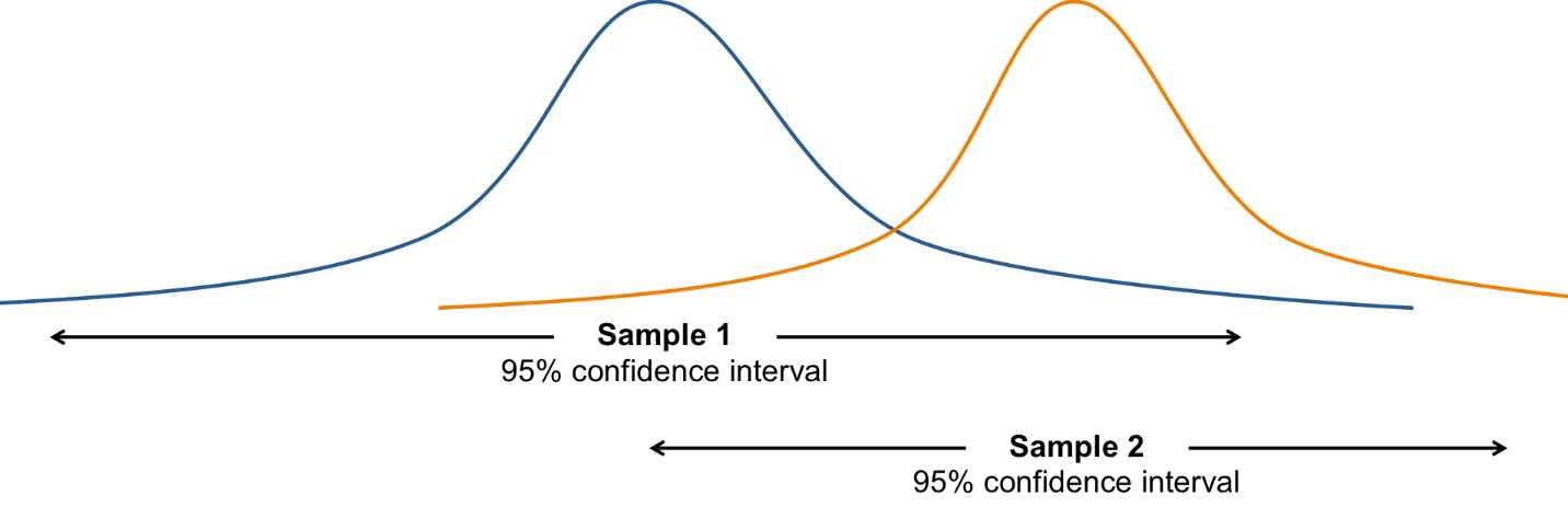
Figure 36: These samples might come from the same population, and the sample means differ simply due to chance.

We use a t-test to decide if the samples are statistically different or if they differ due to chance. We have two independent samples, each with their own standard deviations, which means we need to pool the standard deviations together to calculate the standard error. The t-statistic becomes:

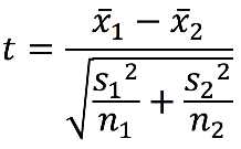
Essentially, this determines whether or not the difference between sample means is significantly different than 0 (similar to the one-sample t-test):

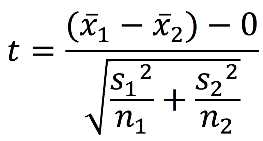
Because we have two different sample sizes, the degrees of freedom is the sum of the individual degrees of freedom: n₁ + n₂ – 2.

Example

Let’s say we want to test whether or not a gender wage gap exists for independent contractors. If we perform a two-tailed test, our null and alternative hypotheses are:

H₀: m_M – m_F = 0
H_a: m_M – m_F ¹ 0

Here m_M is the population of male contractors’ hourly rates, and m_F is the population of female contractors’ hourly rates.

We take a random sample of 17 male and 15 female independent contractors and find each person’s hourly rate. Then we calculate each mean and sample standard deviation.

Males
_M = $37
s_M = $18

Females
_F = $33
s_F = $12

Therefore, the t-statistic is

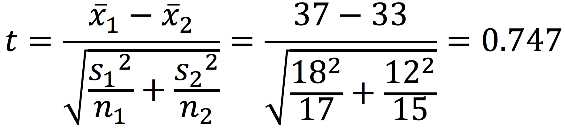
with df = 30.

The t-table tells us that t_{(0.05, 30)} = 2.042 for a two-tailed test. In other words, the t-critical value marking the bottom 2.5% and top 2.5% is ±2.042. In this case, we fail to reject the null, and we conclude that there is no significant difference between male and female independent-contractor hourly rates for these two populations.

Tip: We never say that we “accept“ the null because we don’t truly know if the null hypothesis is true. To know this, we would need to know information for the entire population. Instead, we’re basing conclusions off of a sample that only supports the conclusion that we don’t have enough information to reject the null just yet. So, the proper way to write our conclusion is that we “fail to reject the null.“

There are ways to do an independent-samples t-test in R:

• t.test(a, b)
  In this case, “a” and “b” are arguments for a set of numerical values. For example, a = {1, 3, 4, 5, 5, 3, 7} and b = {4, 3, 4, 2, 1}. This t-test tells us if the means of “a” and “b” are significantly different.
• t.test(a ~ b)
  This code tells us how values of “a” differ by values of “b,” where “b” is categorical.

We can use the code t.test(a ~ b) for our NCES data to determine if people who worked during high school had a higher income in 2011 than those who did not work. Let’s explore this data with a t-test on 2011 income based on whether or not they worked in high school. Since socioeconomic status (SES) may have played a role in people’s decision to work during high school, let’s further explore the data with another t-test on SES based on whether or not they worked.

Our null and alternative hypotheses for a two-tailed test are:

H₀: μ_{income: work} = μ_{income: did not work}
H_a: μ_{income: work} ≠ μ_{income: did not work}

H₀: μ_{SES: work} = μ_{SES: did not work}
H_a: μ_{SES: work} ≠ μ_{SES: did not work}

Code Listing 10

Our results show that students who worked during high school (coded “1”) had higher incomes in 2011 and that the results are significant at p < 0.001. Therefore, in this case we reject the null hypothesis and can conclude that students who worked in high school later earned higher incomes.

However, our second t-test reveals that SES was not significantly different between those who worked and didn’t work during high school, so SES was not a factor in whether or not students chose to work. These findings support the first hypothesis: that students who worked during high school had a stronger work ethic, and as a result they made more money 10 years later.

Now that you’ve learned how to tell if two samples are significantly different, you’ll learn how to discern if any two samples in a group of three or more samples are significantly different.