Standardizing

Use distributions to find probabilities

In the previous chapter, we looked at converting normal distributions into the standard normal distribution (m = 0, s = 1) so that we don’t have to integrate the PDF to calculate probabilities. This process of converting any normal distribution into a standard normal distribution is called standardizing. It allows us to compare two different normal distributions. Specifically, say you are analyzing a value from one normal distribution along with another value on a different normal distribution. How would you know which value is farther from the norm, based on the distribution it comes from? That’s what you’ll learn in this chapter.

Consider the following distribution with m = 15 and s = 3.

Figure 16: This curve is the PDF for a normal distribution with a mean of 15 and a standard deviation of 3.

How would we convert this into a standard normal distribution (mean = 0 and standard deviation = 1)?

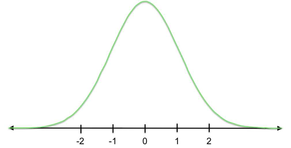
Figure 17: This curve is a standard normal distribution N(0,1), which has mean 0 and standard deviation 1. When we standardize normal distributions, we convert them into the standard normal distribution.

To put the question another way, let’s say that 21 is one of the values in the original data set. If we shift and shrink the distribution to become standard normal, what new value will 21 have?

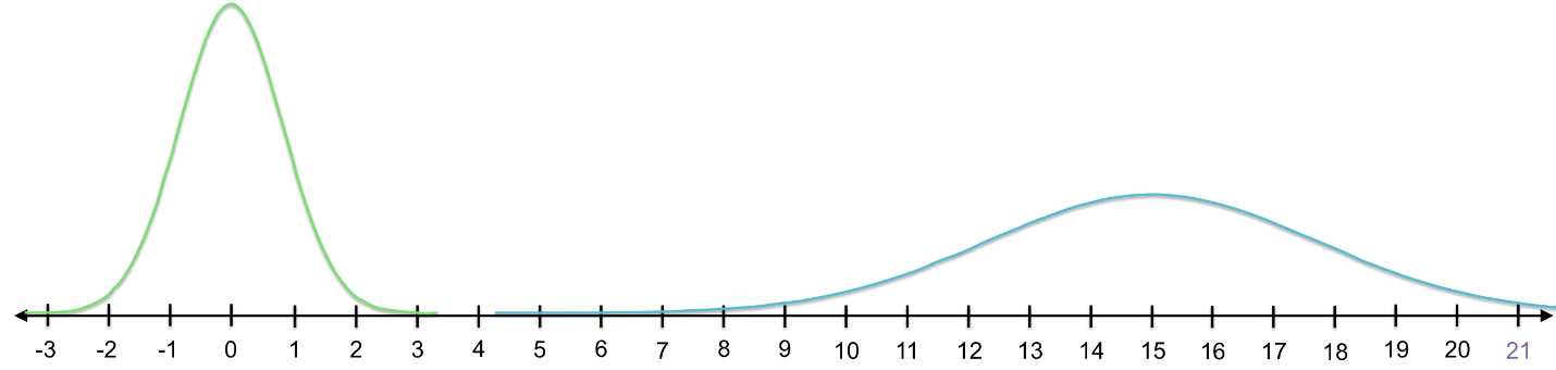
Figure 18: If we want to standardize the blue curve, we need to develop a system for converting it into the green (standard normal) curve.

You might have guessed that we first need to subtract the mean from 21. More broadly, in order to convert the entire distribution into the standard normal distribution, we first must subtract the mean from each value in the data set (x_i - m). This shifts the data to the left so that the new mean is 0.

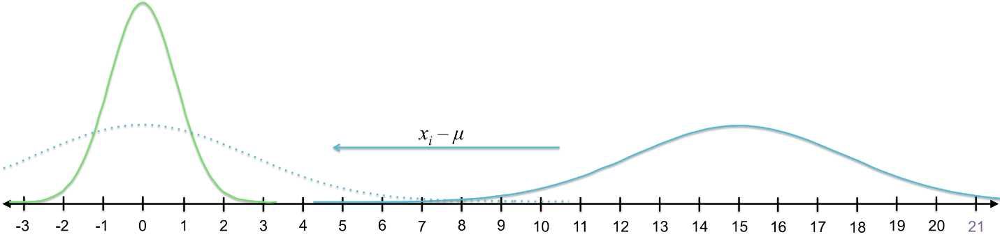
Figure 19: To convert the blue curve on the right into the green (standard normal) curve on the left, we subtract the mean of the blue distribution from each value in the distribution (shifting the entire distribution to have a mean of 0) and then divide by the standard deviation (shrinking the distribution to match the green distribution).

You can see that the new value for 21 would be 6.

Now the mean of each distribution is the same, but the standard deviation of our original data set is 3 and we want it to be 1. So, how can we shrink the spread? We divide by the standard deviation. The standardized value of 21 is therefore (21-15)/3 = 2.

In our original data set, 21 is two standard deviations from the mean (recall the standard deviation is 3 and the mean is 15). When we standardize 21 and it becomes 2, it remains two standard deviations from the mean (now the mean is 0 and the standard deviation is 1).

Think of standardizing this way—you’re simply calculating the number of standard deviations a value is from the mean. This number is called the z-score, denoted z.

Values from different normally distributed data sets with the same z-score will have the same probability of being selected. In other words, the area under the curve that is greater than or less than values with the same z-scores is the same. This is because the total probability under any PDF is 1.

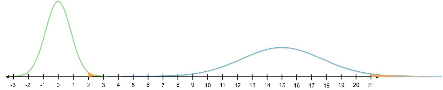
Figure 20: The area under the standard normal curve above 2 is equal to the area under the original curve (m = 15, s = 3) above 21. Both 2 and 21 are two standard deviations above the mean of their respective data sets.

By standardizing distributions and finding z-scores for each value of interest, we can use the standard normal distribution to calculate all our probabilities (i.e. the areas under the PDF). The z-table located at the end of this e-book lists cumulative probabilities for any z-score.

The numbers in the body of that table are the cumulative probabilities (p) less than a particular z-score. For example, the probability of randomly choosing a value less than z = 1.22 is 0.8888 (i.e. P(x < 1.22) = 0.8888).

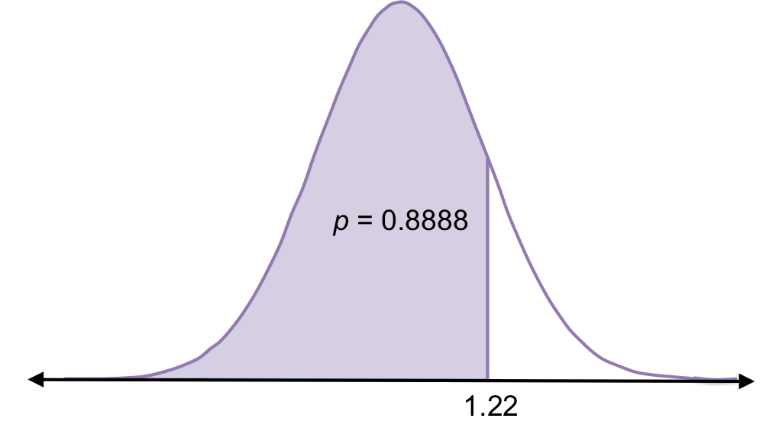
Figure 21: In the standard normal curve, the probability of randomly selecting a value less than 1.22 (i.e. 1.22 standard deviations above the mean) is 0.89.

Note: In probability notation, we usually use x to denote the value of the variable. Note that in this example, because our values of interest follow a standard normal distribution, the x-values are also z-scores.

Upon looking at the z-score table, you’ll see that it shows only cumulative probabilities for positive z-scores. However, since the normal distribution is symmetrical, you can also use this table to calculate probabilities for negative z-scores. For example:

P(x > -1.22) = 0.8888
P(x < -1.22) = 1 – 0.8888 = 0.1112

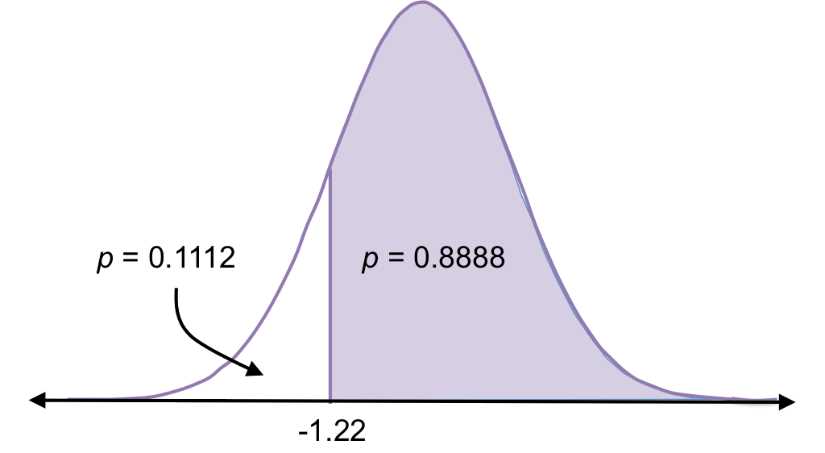
Figure 22: Because normal distributions are symmetric, the probability of randomly selecting a value less than +1.22 is the same as randomly selecting a value greater than -1.22, which is 0.89. All probabilities under the curve add to 1, which means the probability of randomly selecting a value greater than +1.22 is
1 – 0.89 = 0.11, and this is the same as the probability of selecting a value less than -1.22.

Now you know how to do basic statistical analyses. Given any data set, you can describe it, visualize it, and calculate the probability of a particular range of values occurring (using the z-table for normally distributed data or using the PDFs to model data of other distributions).

Let’s now work through a simple real-world example.

Example

You want to take guitar lessons. Somehow you know that the hourly rate for guitar teachers in your area is normally distributed with μ = $28 and σ = $4.6. If you look at a list of guitar teachers’ contact info and randomly choose one to call, what is the probability that this teacher charges between $15 (the minimum for getting a decent teacher) and $25 (the maximum you’re willing to pay)?

First, we’ll standardize the distribution by finding the z-scores for $15 and $25. Because this price range is below the mean, we will expect negative z-scores.

So, you want to find the area under the standard normal curve between -2.83 and -0.65. In other words, you’re looking for the probability of randomly selecting a value between -2.83 standard deviations from the mean and -0.65 standard deviations from the mean.

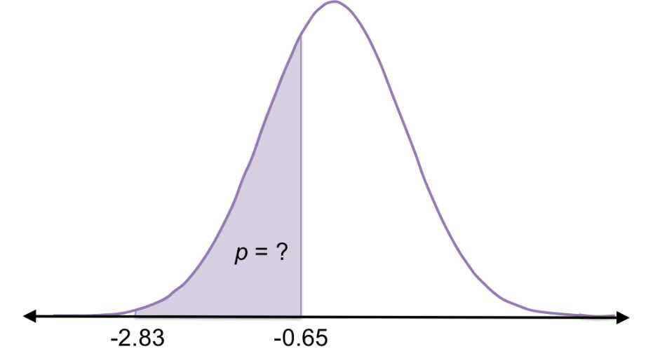
Figure 23: You can use the z-table to find the probability of randomly selecting a value between -2.83 and -0.65 standard deviations from the mean for a normal distribution.

Now you can use the z-table to find the cumulative probability less than positive 2.83, then subtract the cumulative probability less than positive 0.65. Because the normal distribution is symmetric, this is the same probability depicted in Figure 23.

P(x < 2.83) = P(x > -2.83) = 0.9977
P(x < 0.65) = P(x > -0.65) = 0.7422
P(0.65 < x < 2.83) = P(-2.83 < x < -0.65) = 0.9977 – 0.7422 = 0.2555

Therefore, the probability of randomly selecting a guitar teacher who charges between $15 and $25 per hour is about 0.2555, or 25.55%. That means you’d likely find a guitar teacher after four phone calls.

Determine what is significantly unlikely

The shape of the normal distribution—high frequencies around the mean, median, and mode and low frequencies in the tails—allows us to determine if something weird is going on with a particular value or sample (i.e. if we randomly selected a value or sample that is extremely unlikely to be randomly selected).

There are many situations in which we might want to statistically determine if a value is significantly different from the mean. One area is in health: for example, knowing if your heart rate or cholesterol levels are unhealthily high or low.

In normal distributions, a majority of values (about 68%) lie within 1 standard deviation of the mean and almost all (about 95%) lie within 2 standard deviations of the mean.

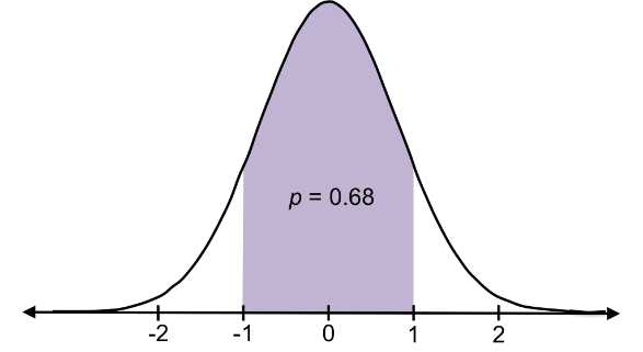
Figure 24: In normal distributions, about 68% of values lie within one standard deviation of the mean, and about 95% of values lie within two standard deviations of the mean.

Therefore, randomly selecting a value more than two standard deviations from the mean in either direction is very unlikely. Generally, we decide that something is statistically unlikely if the probability of selecting a value is less than 0.05. It’s even more unlikely to occur if the probability is less than 0.01, and really really unlikely if the probability is 0.001. These probabilities (0.05, 0.01, and 0.001) are known as alpha levels (a), also called significance levels because if the probability of selecting a value or sample is less than a, the results are considered “significant.”

For example, in the guitar-lesson example, the z-score for $15 is -2.83. This is more than two standard deviations below the mean, i.e. finding a guitar teacher who charges $15 per hour or less is statistically unlikely.

Determining whether or not a probability is less than a is called hypothesis testing. This chapter covers z-tests: hypothesis testing when we know population parameters m and s. For this test, we continue using the z-table. (When we don’t know population parameters, we have a different distribution and use a different table. This will be the focus of Chapter 6.)

We can use three types of hypothesis tests:

• Left-tailed test
• Right-tailed test
• Two-tailed test

All tests use the same alpha levels; however, each has a different location for the cutoff between what is considered significant or not. A left-tailed test analyzes whether or not a value or sample falls significantly below the mean (i.e. in the bottom a); a right-tailed test analyzes whether or not a value or sample falls significantly above the mean (i.e. in the top a); and a two-tailed test analyzes whether or not a value or sample is significantly different from the mean in either direction (i.e. in the bottom a/2 or top a/2).

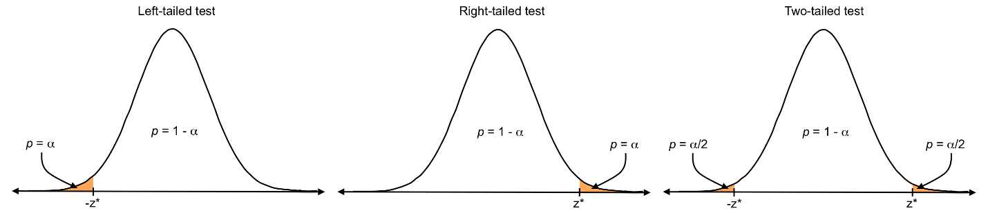
Figure 25: Z-critical values (z*) mark the cutoff for the critical region, which adds to a.

In Figure 25, the orange areas are the critical regions, and the cutoff is the z-critical value, which is based on the chosen a level. If a value or sample falls in the tail beyond the z-critical value, the results are considered significant.

We choose which test to run (left-tailed, right-tailed, or two-tailed) based on our hypothesis. If our hypothesis states that a particular value will be significantly less than the mean, we do a left-tailed test. If we’re not sure, or if we merely speculate the value will be different, we do a two-tailed test.

Let’s calculate the z-critical values for a two-tailed test at each a level. You can see from the z-table that for an a level of 0.05, a proportion of 0.025 is in each tail, and therefore the z-critical values are ±1.96. We then say that if a value has a z-score less than -1.96 or greater than 1.96, it is statistically significant at p < 0.05.

What are the z-critical values for alpha levels of 0.01 and 0.001 for a two-tailed test? Well, 0.01 split between the two tails of the distribution indicates that 0.005 (0.5%) is in each tail. That means the cumulative probability up until the z-score marking the top 0.5% is 0.995. If you find that p = 0.995 in the body of the z-table, you will see that the corresponding z-score is about 2.58. So, ±2.58 is the z-critical value for a = 0.01. Likewise, ±3.27 is the z-critical value for a = 0.001. The most common alpha level used to test for significance is 0.05.

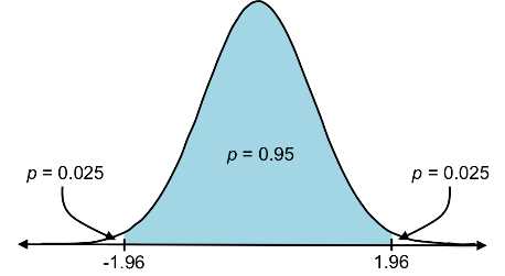
Figure 26: Z-critical values for alpha levels of 0.05, 0.01, and 0.001 are ±1.96, ±2.58, and ±3.27.

Moving forward, we’ll use this concept to estimate the population mean given a sample.