One-Sample Z-Test

Calculate the likelihood of a random sample

Along with comparing individual values to others from the same normal distribution, we can compare a sample of values to other samples from the same population. This will help us determine if a particular sample we have collected is unlikely to occur. We test this essentially the same way we tested in Chapter 4. However, this time, because we have a sample, we look at where the mean of that sample falls in the distribution of means we would get from all other samples of the same size from that population. This distribution of sample means is called the sampling distribution.

If you collect a sample of size n from a population and calculate the mean (₁), then take another sample of size n from the same population and calculate the mean again (₂), and do this as many times as you possibly can so that each sample consists of a unique combination of values from the population, the sample means form a normal distribution. (Generally, sample sizes should be larger than 5.) Amazingly, it doesn’t matter what the distribution of the population is. The population might have a bimodal, uniform, or skewed distribution, yet the sampling distribution will be normal (as long as the sample size—i.e. the number of values in each sample—is greater than 5). This phenomenon is called the Central Limit Theorem.

The sampling distribution is the distribution of all possible sample means of size n. Of course, this is theoretical; we can’t possibly take every possible sample and find the mean. For example, if a population has 100,000 values and we have a sample size of 30, there would be

unique samples of size 30. This number would be ridiculously huge. However, by knowing what the sampling distribution would be if you could take every possible sample of size n, you can tell if something weird is happening with a particular sample.

The mean of the sampling distribution, which we’ll call m_M (i.e. the mean of the means), is equal to the population mean m, and the standard deviation of the sampling distribution (s_M) is equal to s / Ön (the population standard deviation divided by the square root of the sample size). The standard deviation of the sampling distribution is called the standard error (SE).

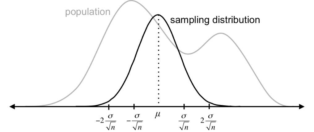
Figure 27: No matter the shape of the population, sampling distributions will follow a normal distribution as long as the sample size is greater than 5. The mean of the sampling distributions is equal to the mean of the population (m = m_M), and the standard deviation of the sampling distribution (the standard error) is the population standard deviation divided by the square root of the sample size (s_M = s / Ön).

Since sampling distributions are normally distributed, about 68% of sample means fall within one standard error (s / Ön) of the population mean, and about 95% fall within two standard errors (2s / Ön). Therefore, it is very unlikely you’ll get a random sample whose mean is more than two standard errors from the population mean in either direction. If this happens, something has probably been done to influence that sample.

When we conduct hypothesis testing for samples, we can test whether or not a particular sample mean is significantly different than the population mean m, or from a particular value, or from another sample. The remainder of this chapter covers how to compare a sample mean to a specific value when we know population parameters m and s. This is called a one-sample z-test.

If the mean of a particular sample is significantly different from the mean of the population from which the sample was taken (m), we assume that something has been done to influence the sample. If all values in the original population were similarly influenced, the entire population would shift to a new mean (m_S), but the standard deviation would remain the same. (Some call the new population’s mean m_I for “influence” or “intervention.”)

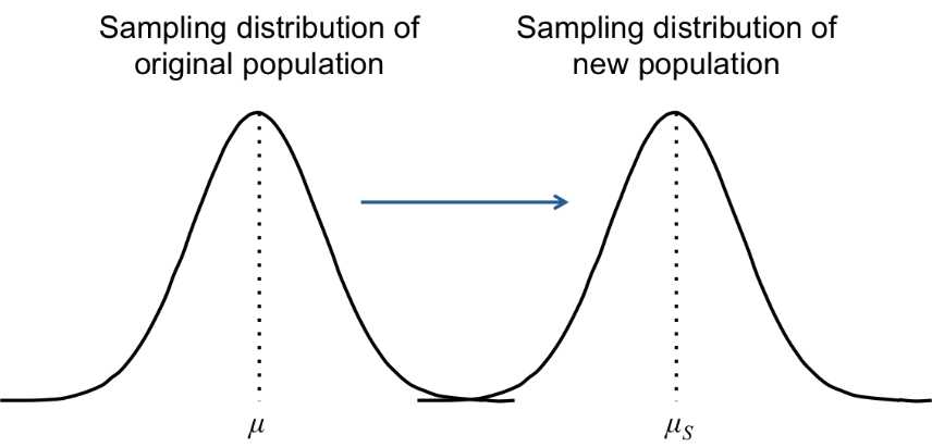
Figure 28: If the mean of a particular sample is significantly different from the mean of the population from which the sample was taken (m), we assume that something has been done to influence the sample. If all values in the original population were similarly influenced, the entire population would shift to a new mean (m_S), but the standard deviation would remain the same.

Our hypothesis test will produce one of two results: either the sample is not significantly different from m, or it is. These two outcomes are called the null and alternative hypotheses. The null hypothesis states that the new population mean, based on the sample mean, is not significantly different from m, and we notate this as such:

H₀: m_S = m

The alternative hypothesis states that the new population mean is significantly different, either by being significantly greater than the mean, significantly less than the mean, or one of the two:

H_a: m_S < m
H_a: m_S > m
H_a: m_S ¹ m

When there is a significant difference, scientists will typically attempt to determine why that difference exists. They can do this through further quantitative analysis, qualitative research, or both.

We use the first two alternative hypotheses when we perform a one-tailed test (H_a: m_S < m for a left-tailed test and H_a: m_S > m for a right-tailed test) and the third alternative hypothesis for a two-tailed test.

Figures 29-31: The purple areas on each distribution depict the critical regions for a = 0.05. If the sample mean falls in the critical region determined by the test, you’re doing (one-tailed or two-tailed), the results are significant.

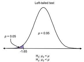
Figure 29

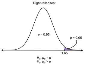
Figure 30

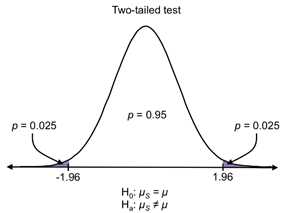
Figure 31

Example

Let's say a particular regional gym in the U.S., one with about 6,000 members, hires you to estimate the health of its membership so that it can boast of being an effective gym. You decide to use resting heart rate as an indicator of health, where the lower the resting heart rate, the healthier the individual.

You know from research that for all people in the United States aged 26-35, the mean resting heart rate is 73 with standard deviation 6. When you take a random sample of 50 gym members aged 26-35, you find that their average resting heart rate is 68. Can you say that members of this gym are healthier than the average person?

To answer this question, let’s first write out the null and alternative hypotheses.

H₀: m_S = 73
H_a: m_S ¹ 73

In order to determine whether to reject or accept the null hypothesis (that there is no significant difference in health between people at this gym and the general population), describe the sampling distribution of all samples of size 50 from the population of US adults aged 26-35. The mean is the same as the population mean (73) and the standard error is s / Ön = 6 / Ö50 = 0.85. Where on this distribution does the sample mean (68) lie? In other words, how many standard errors is this particular sample mean from the population mean? We need to find the z-score of the sample mean: 

You can see from the z-table that the probability of selecting a random sample from the population of 26-35-year-olds with a mean of 68 is about 0. Therefore, we can say that our results are statistically significant, with p < 0.001 (our smallest alpha level). We reject the null and conclude that the sample comes from a different population. In layman’s terms, people at this gym are healthier than the average person.

(Of course, it could be that healthy people self-select to be members of this gym, and the gym isn’t causing them to be healthier. To differentiate correlation—how two data sets change together—versus causation—whether or not one data set influences another—we could compare the members’ resting heart rates before they joined the gym to their current resting heart rates. This involves another statistical test, which we’ll examine in the next chapter.)

For now, let’s focus on how to create a function that calculates the z-statistic in R given any mean and standard deviation. The following Code Listing creates this function, then chooses a random sample from the variable “income2011,” then calculates the z-score for that sample.

Code Listing 5

Note: In this example, the z-test returned 0.03 for the z-score. However, when you execute this, you will get a different result because the sample() function in R will generate a different random sample each time.

With the z.test() function you created, you can calculate the z-statistic for any three arguments you input. For example, if “a” is a set of specified values, z.test(a, 5, 3) will calculate the z-score for the mean of “a” on a sampling distribution that has mean 5 and standard deviation 3.

Find a range for the true mean

Once you determine that a sample is significantly unlikely to have occurred and therefore most likely comes from a new population with mean m_S, you can determine a range in which you’re pretty sure m_S lies. You can assume that this population has the same standard deviation as the original and that some kind of intervention has merely shifted the population one way or another.

Your best guess for m_S is , but because you know that 95% of sample means are within 1.96 standard errors from the population mean, you can guess the true population mean m_S will be within 1.96 standard errors from . This range is called a 95% confidence interval, and as you saw before, 1.96 is the z-critical value that marks the middle 95% of the data.

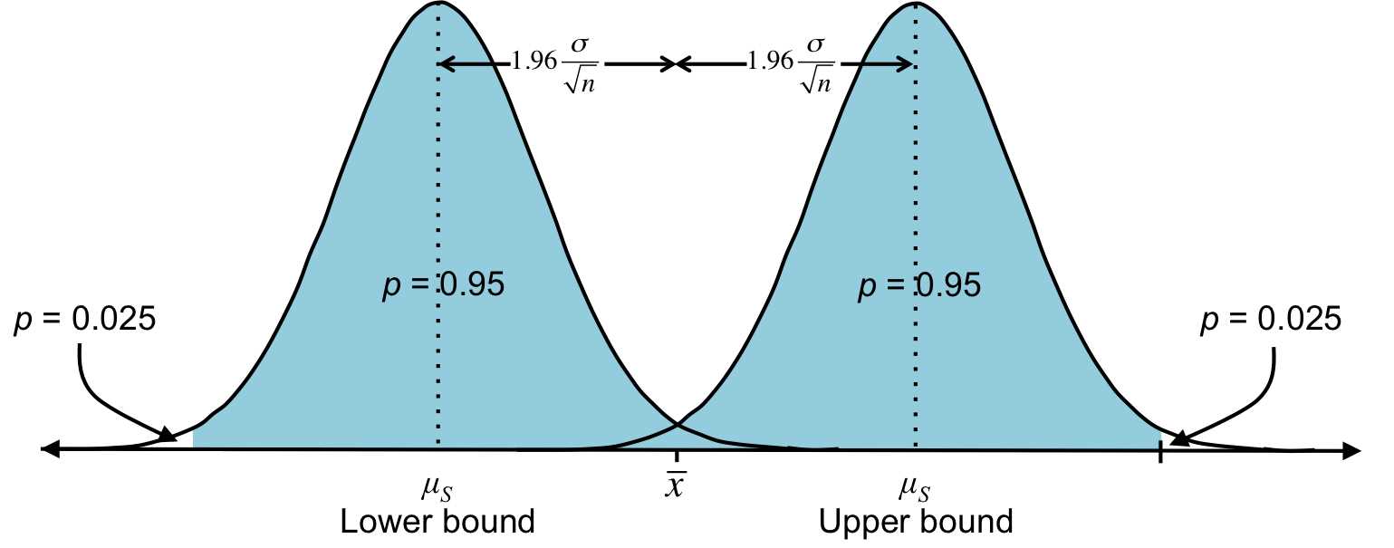
Figure 32: Each distribution above is the same sampling distribution consisting of all samples of size n. And is the mean of a sample of size n. Most likely, this sample is one of the 95% within two standard errors of the population mean. Therefore, we can calculate a range in which we’re pretty sure m_S lies. This particular range is the 95% confidence interval.

Let’s explore this in the context of our example.

Example

We want to estimate the mean resting heart rate of all members of this gym who are aged 26-35. This is the new population (rather than everyone in the US aged 26-35). The standard deviation of this new population remains the same as the old population: s = 6. 

We found that = 68. Most likely, this sample mean is one of the 95% of sample means that fall within 1.96 standard errors of the population mean. Assuming it is, m_S would fall between

Other confidence intervals

We could also come up with a broader range, such as a 98% confidence interval. In this case, we would be even more certain that m_S is in this range. You can find this interval by first determining the z-critical values that mark the middle 98% of the data. The z-table tells us these values are ±2.33 (since 1% is in each tail). So, you’re pretty sure that the sample lies within 2.33 standard errors of the population mean m_S, which tells us that the 98% confidence interval for m_S:

In general terms, the bounds of a C% confidence interval are

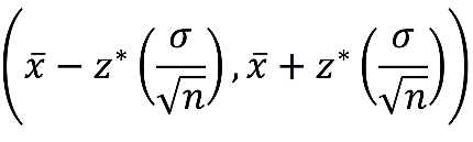
where z* is the z-critical value marking the lower and upper bounds of the middle C% of the distribution.

The following R code creates functions to calculate the lower and upper bounds of a 95% confidence interval. The inputs “sample.income” and “sigma.income” continue from Code Listing 5 and are used to calculate a 95% confidence interval based on the random sample “sample.income.”

Code Listing 6

The sample “sample.income” indicates that the true mean of the population it comes from is between 16,723.69 and 38,226.31. Note that the mean of “income2011” is 27,302. The fact that 27,302 lands smack in the middle of this confidence interval makes sense given that “sample.income” has a z-score of 0.03, which is found in the middle of the sampling distribution.

Calculate the likelihood of a proportion

Along with determining whether or not a sample mean is likely to occur, sometimes we also want to determine if a proportion is likely to occur. For example, if a certain diet plan says that half of people who begin this plan start losing weight after one week and we find that of 30 people, only 11 lost weight after one week, we can execute a test to determine if the proportion who lost weight is significantly less than 50% (which is what we would expect).   

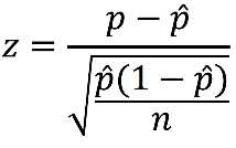
We denote our expected proportion as and the observed outcome as p. So, our general null and alternative hypotheses are:

In this example, our null and alternative hypotheses are:

H₀: p = 0.5
H_a: p ¹ 0.5

To test for significance, we’ll again think about our expected, theoretical sampling distribution. If we take every possible sample of size n from our expected population (in this example, those who participate in this diet plan) and find the proportion of each sample that obtained the result we’re interested in (in this case, those who lost weight after a week), the distribution of sample proportions would be expected to have mean and this standard deviation:

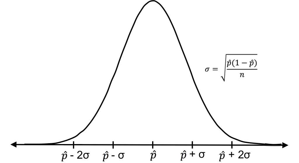
Figure 33: The sampling distribution for sample proportions has mean (which is equal to the population proportion) and standard deviation .

Now that we know the mean and standard deviation of the sampling distribution, we can determine where the observed outcome (p = 11/30 = 0.367) falls on this distribution. This is another z-test.

In our example,

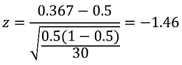
the result is greater than the z-critical value on the left tail of -1.96. Therefore, the results are not significant, i.e. the proportion of those who lost weight is not significantly less than 0.5. This diet plan’s claim could still be true!

Let’s now preform a test for proportions using the NCES data. Perhaps we want to know if the proportion of students who worked while in school is significantly more or less than 0.5. Again, we’ll create a function that returns the z-statistic.

Code Listing 7

Now you can use the p.test() function for any set of binary data to test whether the proportion of one of the values significantly differs from any specified proportion—in this case 0.5. As you can see from the z-score of -20.9, the result of this particular test reveals that the proportion of students who worked during high school is significantly less than 0.5.

By now, you should be comfortable calculating probabilities under the normal curve and using these probabilities to determine if a value, sample, or proportion is out of the ordinary. In the next chapter, we’ll look at which kinds of test to execute when you don’t know original population parameters m and s.