Central Tendency

Calculate measures of center

Central tendency is a term that describes one point at which a group of values gathers.  Measures of center are statistics that describe the central tendency. You’ve probably heard of the three most commonly used measures of center: mean, median, and mode. This chapter will define and describe how to calculate each. It is important to know what they are, and it is also important to know what they mean, especially in relation to each other. By looking at how the mean, median, and mode compare to each other, we can better understand the story the data is telling.

Mode

The mode is where most of the numbers in a data set occur, i.e. where the frequency is the greatest. This could be a single number or a group of numbers. For example, in the small data set {2, 3, 3, 4, 6}, the mode is 3 because the frequency is 2 (3 appears twice), while the frequency of the other values is 1.

A histogram is the most common way to visualize the mode of a distribution. A histogram is a special type of bar graph that shows the values in the data set on the x-axis and the frequency of those values on the y-axis. Values on the x-axis are grouped into bins of a specified range or category.

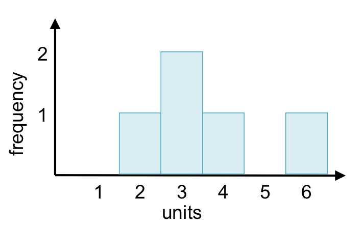
Figure 1: A histogram of the data set {2, 3, 3, 4, 6} shows that the mode is 3.

The mode doesn’t have to be a number. For example, let’s say in the local high school biology class, 10% of students scored A’s, 40% scored B’s, 35% scored C’s, and 15% failed. In this case, the mode is a grade of B. This type of data set is an example of categorical data (as opposed to numerical data), in which data is arranged in categories (in this case, the grade in the class).

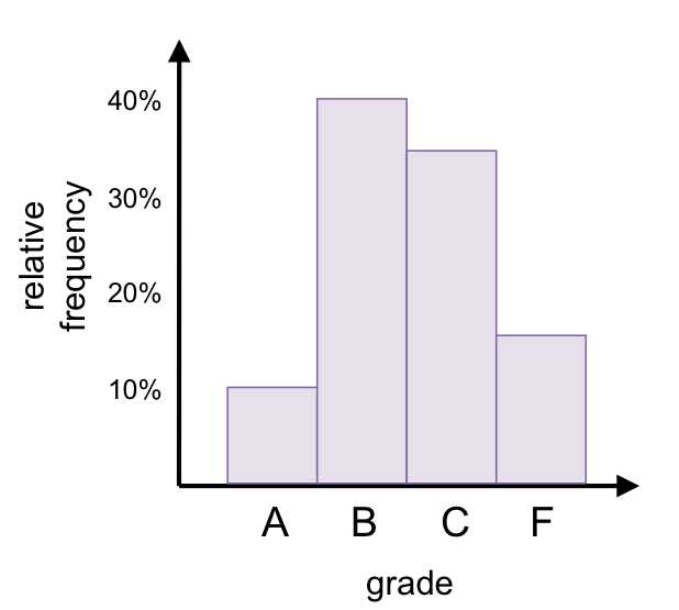
Figure 2: In this categorical data set, the mode is a grade of B.

Note: The y-axis in Figure 2 shows the relative frequency—the frequency of each category in relation to one another—rather than the absolute frequency, which would depict the absolute number in each category.

For large, continuous data sets, the mode is the range with the highest frequency. The following histogram shows ten bins, each with a width of 5 units. You can easily see that the mode is the range (35, 40). Remember that the mode is where the greatest frequency occurs (the values along the x-axis), not what the frequency is (i.e. the mode is not 8).

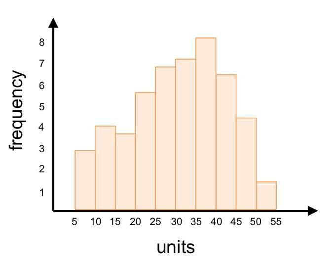
Figure 3: The mode of the data set visualized by this histogram is the range (35, 40).

Median

The median is another measure of center. This statistic is a number for which 50% of the values in the data set are less and 50% are greater. In the case of a data set with an odd number of values, the median is an actual value in the data set and is smack dab in the middle. For example, the data set {5, 6, 8, 12, 15} has a median of 8. Two values are less than 8 and two values are greater than 8.

When a data set has an even number of values, the median is the average of the two middle numbers. The median of the data set {4, 6, 9, 11, 17, 18} is 10—the average of 9 and 11. Three values are less than 10 and three values are greater than 10.

You may have noticed that values must be ordered; otherwise the median can’t be computed. Also note that we can’t find the median for categorical data, but we can for numerical data.

Note: Unlike the mode, we can’t easily see where the median is by looking at a histogram. We need to put the values in order and find the middle number(s).

Notice that the numbers less than or greater than the median can be anything (so long as they remain less than or greater than the median) and the median will remain the same. For example, the following data sets all have the same median:

{5, 6, 8, 12, 15}

{5, 6, 8, 20, 300}

{-100, -16, 8, 12, 15}

{-100, -16, 8, 20, 300}

Therefore, the median by itself does not adequately describe a data set.

It’s also helpful to have a statistic that accounts for every value. This is why a more common measure of center is the mean.

Mean

Unlike the mode and median, the mean (also known as the arithmetic mean) uses every value in the data set in its calculation.

Note: Other types of means exist (e.g., geometric mean, harmonic mean), but the arithmetic mean is the most common. It is “arithmetic” because it’s calculated by adding every value in the data set and then dividing by the number of values.

For a data set {x₁, x₂, x₃, … x_n}, where n is the number of values in the data set, the mean is represented by x (x-bar) and is equal to:

We can rewrite this as:

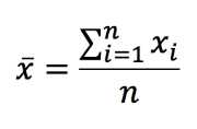
The Greek letter capital sigma (Σ) symbolizes taking the sum. The i = 1 and the n on the bottom and top of Σ indicate the values of i that we should use in the summation: 1, 2, 3, … n. So, we should substitute the subscript i from x_i with 1, 2, 3, all the way to n (where n could be any number). This translates to finding the sum of x₁, x₂, x₃, all the way to x_n. Then we divide the sum by n to find the mean.

We use the symbol (x-bar) to represent the mean of a sample and the symbol m (mu) to represent the mean of a population. In general, we use lowercase letters when describing a sample and uppercase letters when describing a population (x_i are values of a sample and n is the sample size, while X_i are values of a population and N is the population size). Therefore, the mean of a population is represented by:

Note: If you’re wondering why statistical notation must be so complicated, you’re not alone. But once you get the hang of it, this language is a very useful tool for quickly and easily communicating complex statistical ideas.

Because the mean uses every value in its calculation, outliers (values in the data set that differ significantly from other values in the same data set) can severely affect it. Take the two data sets below, one of which has an outlier:

{4, 6, 7, 10}      = 6.75

{4, 6, 7, 100}    = 29.25

This example illustrates why the mean is not always the best measure of center. If we only know the mean of the second data set, we would think that the values cluster around 29.25, when in fact 75% of them are less than 8.

When the mean, median, and mode for a data set are roughly equal, the mean is used to calculate many other statistics (e.g., how spread out the data is) to perform a multitude of analyses. For this reason, the mean is the most common measure of center.

Let’s look at how to find the mean, median, and mode in R using the NCES data. (If you have not yet downloaded the data, imported it into R, and run the attach() function, do this first.)

Code Listing 2

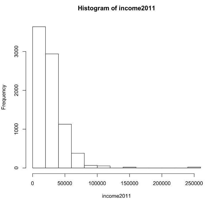
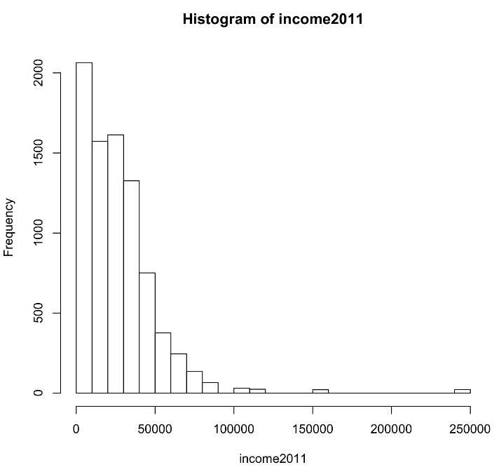
You can see that the variable “income2011” is heavily skewed (i.e. most values fall on one side of the full range of the data). The majority of students have a family income of less than $50,000.

This skewedness results in the mean being greater than the median. Recall that the median is not influenced by outliers because it is the exact middle value, while the mean is affected by every value in the data set. In this case, outliers (students with a family income of $250,000) are pulling the mean to the right. When the mean differs from the median, it suggests the presence of outliers and a skewed distribution such as the one in this example.

Taken together, the mean, median, and mode can provide a useful description of a data set. In the next chapter, you’ll learn methods to calculate the variability of a data set—in other words, how “spread out” values are in relation to each other. When describing data, the variability is as important as the measures of center.