ANOVA

---

Test for differences between three or more samples

When we have three or more samples and we want to determine if any two of them are significantly different from each other, we utilize a statistical test called analysis of variance (ANOVA). This test analyzes how a dependent variable differs based on one or more independent variables. For example, we may want to know if scores on a standardized math test (the dependent variable) are significantly different between students who go to School A, School B, and School C (where school is the independent variable).

The dependent variable should be continuous (math test scores are continuous), be approximately normally distributed, and have homogenous variances for the values for each of the groups. The independent variable should be categorical with mutually exclusive values (where “School A,” “School B,” and “School C” are the different values). The independent variable should also be approximately normally distributed.

This chapter covers both one-way and two-way ANOVA. In one-way ANOVA, there is one independent variable; in two-way ANOVA there are two independent variables.

Compare samples based on one factor

The null and alternative hypotheses are:

H₀: μ₁ = μ₂ = … = μ_k
H_a: at least two population means are significantly different

where there are k samples.

This test involves measuring between-group variability—essentially, the variance of the sample means—and dividing between-group variability by a measure of within-group variability—a combined measure of each sample’s variance. The resulting quotient is the F-statistic.

F = (between-group variability) / (within-group variability)

The greater F is, the more likely at least two populations are significantly different. If you think about this quotient, greater between-group variability indicates that the sample means are spread out farther from each other, which implies they’re more likely to be significantly different.

Smaller between-group variability

Greater between-group variability

Figure 37: In the previous figure, within-group variability is the same, but between-group variability changes. As between-group variability increases, samples are more likely to be significantly different and the F-statistic increases.

On the other hand, greater within-group variability indicates that the standard deviation of each sample is greater, which implies the samples are less likely to be significantly different.

Smaller within-group variability

Greater within-group variability

Figure 38: In this figure, between-group variability is the same, but within-group variability changes. As within-group variability increases, samples are less likely to be significantly different and the F-statistic decreases.

So, the greater the numerator (between-group variability) and the smaller the denominator (within-group variability), the greater the F statistic will be. Let’s calculate each of these in turn.

Between-group variability

Measuring the spread of sample means is just like calculating the variance. First, we find the grand mean (_G), which is the sum of all values from each sample divided by the sum of each sample size.

In the first expression, x_1i represents all values from sample 1, x_2i represents all values from sample 2, etc., while n₁ is the size of sample 1, n₂ is the size of sample 2, etc., for k samples; in the second expression, j is the sample number that ranges from 1 to k, while i is the value number in each respective sample.

To calculate between-group variability:

1. Calculate the deviation of each sample mean from the grand mean: .
2. Square each deviation: .
3. Multiply each squared deviation by the sample size of that respective sample to weigh the squared deviation by the sample size: .
4. Sum each weighted squared deviation: .
   This gives us the sum-of-squares for between-group variability (SS_between).
5. Find the average squared deviation by dividing SS_between by the degrees of freedom, where df_between = k – 1. This quotient is known as the mean square for between-group variability (MS_between), and this is our final measure of between-group variability.

.

Within-group variability

This is a measure of error that combines the error within each individual sample. To calculate within-group variability:

1. Calculate the deviation of each value from the mean of the sample it comes from: .
2. Square each deviation: .
3. Sum the squared deviations: .
   We now have the sum of squares for within-group variability (SS_within).
4. Find the average squared deviation of each value from its respective sample mean by dividing SS_within by df_within (the sum of the degrees of freedom of each sample), where df_within = (n₁ - 1) + (n₂ - 1) + … + (n_k - 1) = n₁ + n₂ + … + n_k - k = N – k. This quotient is the mean square for within-group variability (MS_within) and is our final measure of within-group variability.

Total variability

If we take the deviation of each individual value from the grand mean, square each deviation, and find the sum of squared deviations, we get the total sum-of-squares (SS_total), a measure of the total variability. What’s cool is that SS_total is the sum of SS_between and SS_within.

SS_between + SS_within = SS_total

We often organize all our calculations in an ANOVA table.

Table 5: ANOVA tables help organize variability calculations.

The F-distribution

As with z- and t-statistics, F-statistics follow a specific distribution. In our calculation of between- and within-group variability, we (essentially) found average squared deviations. Therefore, F can never be negative, and the distribution lies along the positive x-axis.

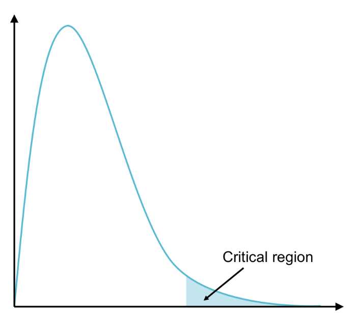
Figure 39: The F distribution has one tail on the right (on the positive x-axis). The critical region lies in this tail.

This also makes sense in the context of what we’re testing for—we simply want to know if at least two populations are significantly different, not if one is significantly less than or greater than another.

Once we’ve calculated the F-statistic, we use the F-table to determine the F-critical value,
F(α, df_between, df_within). You’ll see in the F-table that the column headers are df_between and the row headers are df_within. A specific F-table exists for each alpha level.

Example

As a digital marketer, you always try to determine the most effective means of advertising online. Let’s say you’ve placed ads with a number of online publications, in various locations on each web page, and you decide to perform ANOVA to determine if different locations have better click-through rates (CTR, which is the ratio between the percentage of users who click the ads and the total site visitors). The three most common ad locations are on the top, middle, and sides of the page. In your research, you find the CTR of more than 600 ads.

Table 6: This ANOVA table helps organize between-group and within-group variability calculations.

This gives us everything we need to calculate between-group and within-group variability.

Between-group variability:

We know that:

And therefore,

This leads us to SS_between = (35 – 34.1)² + (28 – 34.1)² + (38 – 34.1)² = 53.23

We also know the degrees of freedom for between-group variability (df_between) = 2 (because there are three categories for our independent variable (top, middle, sides) and we subtract 1.

Now we can find between-group variability.

Within-group variability:

By knowing each sample’s sum-of-squares, we can find SS_within.

= 3.2²(235 – 1) + 4.3²(169 – 1) + 2.5²(210 – 1) = 6808.73

We also know that the degrees of freedom for within-group variability (df_between) equals the total number of values minus the number of categories.

N – k = 235 + 169 + 210 – 3 = 611

Finally, we can find within-group variability (i.e. MS_within) by dividing SS_within by df_within.

F-statistic:

Finally, we can find the F-statistic.

We can organize all our calculations in an ANOVA table. You’ll get the same output when you do an ANOVA test in R, but the SS and df columns will be switched.

Table 7: Results of between-group and within-group variability calculations with F-statistic finding.

Once we’ve calculated the F statistic, we can compare this to the F-critical value
F_{(0.05, 2, 611)} = 3.

Because the F-statistic is less than F_{(0.05, 2, 611)}, the results are not significant. Therefore, we fail to reject the null, and we conclude there is no evidence to suggest any two of the populations—where each population is the CTR for each ad location for all publications—are significantly different. In other words, there is no significant difference between the CTRs of different ad locations on web pages.

Now that we’ve performed one-way ANOVA by hand, let’s execute it in R with the NCES data. Let’s say we want to know if SES differs significantly by race (where subjects are coded 0 if they are “White”—see the Appendix for labels corresponding to other races). We’ll first apply the tapply() function, which tells us the statistic (e.g., mean, median) we will specify for a particular variable as broken out by the other variable. The tapply(ses, race, mean) function will take the mean of SES as broken out by race.

Next, we’ll use the term “fit” to name the ANOVA test, then we’ll summarize “fit” to see the results.

Code Listing 11

You can see from the tapply() function that white students (code = 0) are of higher SES than students of other races. The ANOVA test confirms that these differences are significant because the F-statistic is huge (119). The presence of asterisks (*) also signifies significance.

After determining that at least two populations are significantly different, we can determine which two populations by running a post hoc test. Choosing which post hoc test best suits our needs will be dependent upon our initial data. If our original data has about the same variance (i.e. homogeneity of variance), we can use a test called Tukey’s HSD (for “honestly significant difference”). If not, we can use the Games Howell test. First, let’s go through a test to determine whether or not variances are homogenous.

Levene’s test for homogeneity of variance

In this test, the null and alternative hypotheses are:

H₀: s₁² = s₂² = … = s_k²
H_a: at least two population variances are significantly different.

How the statistic is calculated goes beyond the scope of this e-book; however, you’ll learn how to do this in R.

Because R is open source, people all over the world develop packages containing new functions that perform various statistical tests. For example, the “lawstat” package contains the levene.test() function, and you can install this package in order to run this test for homogeneity of variance.

First, download the package from cran.r-project.org/web/packages/lawstat/. The following code listing explains how to install the package in R and how to run Levene’s test using the ANOVA example of how SES differs by race.

Code Listing 12

Tip: If you’re not sure how to use a particular function in R, you can type a ? followed by the function name, and R will output information on each input of the function. For example, typing ?levene.test() and hitting ’enter’ will show you how to use this function.

According to this test, variances are not homogenous. Therefore, we would use the Games Howell test to determine which students have significantly different SES by race. First, let’s pretend the results of Levene’s test were not significant and go over how we would perform Tukey’s HSD in R.

Tukey’s HSD (variances are homogenous)

The TukeyHSD() test outputs the absolute differences between the means of each group (in this case, the difference between the mean SES), the lower and upper bounds of the 95% confidence interval for these differences, and the p-value (where p-values less than a indicate honestly significant differences).

Code Listing 13

You can see from the results of the Tukey’s HSD test that the only races that do not have significantly different SES levels are between:

• Groups 3 and 1 (“Black or African American, non-Hispanic” and “Amer. Indian/Alaska Native, non-Hispanic”).
• Groups 4 and 1 (“Hispanic, no race specified” and “Amer. Indian/Alaska Native, non-Hispanic”).
• Groups 5 and 1 (“Hispanic, race specified” and “Amer. Indian/Alaska Native, non-Hispanic”).
• Groups 6 and 2 (“More than one race, non-Hispanic” and “Asian, Hawaii/Pac. Islander, non-Hispanic”).
• Groups 5 and 3 (“Hispanic, race specified” and “Black or African American, non-Hispanic”).

However, remember that the data did not pass our homogeneity of variance test, so let’s see what the Games Howell test has to say.

Games Howell (variances are not homogenous)

A package called “userfriendlyscience”[2] includes a convenient oneway() function that can output the results of a number of tests we specify in addition to the ANOVA results, including Levene’s test and the Games Howell test. Let’s run the oneway() function in R and include results of the Levene’s test to compare with the results we got earlier from the “lawstat” package.

Code Listing 14

We get the same results for ANOVA and Levene’s test using the oneway() function. We know from ANOVA that at least two groups are significantly different (i.e. at least two races have different SES levels), and we know from Levene’s test that there is not homogeneity of variance in SES between the different races.

Finally, it turns out that the Games Howell test gives us the same results as Tukey’s HSD.

Compare samples based on two factors

You just learned one-way ANOVA, which compares groups based on one independent variable (i.e. one factor). In our example, that factor was the location of the ad on the web page (top, middle, or sides). The dependent variable was the ad’s click-through rate.

Now let’s work with two-way ANOVA, which tests for significant differences based on two factors. For example, you may want to see how 2011 income differs by gender and whether or not getting good grades as a student differentiates income. Not only are you interested in the difference in income based on gender and grades, but also in a possible interaction effect between gender and grades (i.e. is the difference in income consistent between genders irrespective of grades received and is the difference in income consistent between grades irrespective of gender?).

There are three null hypotheses in two-way ANOVA:

• The means for Factor 1 are equal.
• The means for Factor 2 are equal.
• There is no interaction effect between Factor 1 and Factor 2.

Two-way ANOVA outputs an F-statistic for each hypothesis that determines whether we reject or fail to reject it. Calculating these statistics by hand gets very complicated, so we’ll simply review the basic principles before performing the analysis in R.

Each factor has a certain number of categories (e.g., in the NCES data, the factor “gender” has two categories: “male” and “female”; the factor “grades” has two categories: “Yes” and “No” in regard to whether or not the student was recognized for good grades). Let’s say Factor 1 has k categories and Factor 2 has q categories.

Each category contains a certain number of numeric values. Let’s use n to represent the number of values in Factor 1, where n₁ is the number of values in Category 1 of Factor 1, n₂ is the number of values in Category 2 of Factor 1, etc., through n_k, which is the number of values in Category k of Factor 1.

Let’s use m to represent the number of values in Factor 2, where m₁ is the number of values in Category 1 of Factor 2, m₂ is the number of values in Category 2 of Factor 2, etc., through n_q, which is the number of values in Category q of Factor 2.

Table 8: Two-way ANOVA has two factors (i.e. independent variables). Let’s say Factor 1 has k categories and n total values, and Factor 2 has q categories and m total values.

Our goal in two-way ANOVA is the same as with one-way ANOVA: we want to calculate measures of between-group variability and divide by a measure of error (within-group variability) to calculate our F-statistic. However, this time we’ll calculate two additional F-statistics: one for the second factor and one for the interaction between the two factors. We symbolize this interaction with a multiplication sign.

Let’s first calculate the sums-of-squares for Factor 1 and Factor 2 (SS_between for each), the interaction of Factors 1 and 2 (SS_1×2), the error (SS_within), and SS_total.

We can make these calculations easier by organizing the means of each category in a table.

Table 9: The Mean Table organizes both the mean of each subset based on each factor and the marginal means (the mean of all values in each category of each factor). Marginal means are used to calculate between-group variability, while the means of each bucket (in a specific category of each factor) are used to calculate within-group variability.

_G can also be found by taking the weighted averages of the averages of each category, i.e. by choosing one of the factors, multiplying the average of each category by the sample size, and dividing the sum by N, where N = n₁ + n₂ + n₃ = m₁ + m₂.

You can see we have six buckets of values associated with one of the categories from Factor 1 and one of the categories from Factor 2.

Now we can calculate the sums-of-squares for Factor 1 and Factor 2. SS₁ is found by subtracting the grand mean _G from the mean of each category from Factor 1, squaring each deviation, multiplying each squared deviation by the sample size for that category, and taking the sum. Similarly, SS₂ is found by subtracting _G from the mean of each category from Factor 2, etc.

Note: These equations assume there are k categories for Factor 1 and q categories for Factor 2; however, Table 1 shows that k = 3 and q = 2.

To calculate the sum-of-squares for within-group variability (our error term), subtract the mean of each bucket (Factor 1 Category i and Factor 2 Category j) from each value in that bucket, square each deviation, and take the sum.

Note: Here’s a translation—this equation takes the first value in Factor 1, Category 1 and Factor 2, Category 1 (the top left box in the mean table) and subtracts the mean of all values in Factor 1, Category 1 and in Factor 2, Category 1, then continues this for every value in the data set. In other words, it sums the squared deviations of each value from the mean of all values in that same bucket (Factor 1 Category i and Factor 2 Category j). The above equation for SS_within uses h to represent the h’th value of each category (x_h,1,1 is the h’th value of Factor 1, Category 1 and Factor 2, Category 1).

The total sum-of-squares is the sum of the squared deviations of every value in the data set from the grand mean.

Because all the sums-of-squares sum to SS_total (SS₁ + SS₂ + SS_1×2 + SS_within = SS_total), we can calculate the sum-of-squares of the interaction (SS_1×2) by subtracting SS₁, SS₂, and SS_within from SS_total.

After finding each sum-of-squares, we need to know the degrees of freedom in order to calculate the mean square for each factor (MS₁ and MS₂), the error (MS_within), and the interaction (MS_1×2). The F-statistics will be each mean square divided by MS_within.

Again, it helps to organize these calculations in a table.

Table 10: The ANOVA Table organizes the sums-of-squares (SS) for Factor 1, Factor 2, the interaction (Factor 1 × Factor 2), the error (within-group variability), and in total; the degrees of freedom (df); the mean squares (MS), which is SS/df; and the F-statistics (F), which tell us whether or not values of the dependent variable significantly differ by Factor 1, by Factor 2, or due to an interaction between the two.

This should give you an idea of how we find each F-statistic, which, like one-way ANOVA, is the ratio of between-group variability to within-group variability.

Let’s now perform ANOVA on the NCES data using R with “income2011” as the dependent variable and “gender” and “grades” as the two factors or independent variables. We have coded subjects who are male as 0 and subjects who are female as 1. Subjects with bad grades are coded as 0 and subjects with good grades as 1.

Code Listing 15

We can make a few observations using the tapply() function: males made an average of about $7,000 more than females, and students recognized for good grades made more than $6,000 annually in 2011.

When we perform ANOVA, we see that not only does income significantly differ by gender and whether or not students had good grades—there is also an interaction between these two factors, indicating that income is not consistent between grades when you separate students by gender. We can better understand this interaction effect by finding the mean income for each of the four groups (males who received good grades, females who received good grades, males who did not receive good grades, and females who did not receive good grades).

Code Listing 16

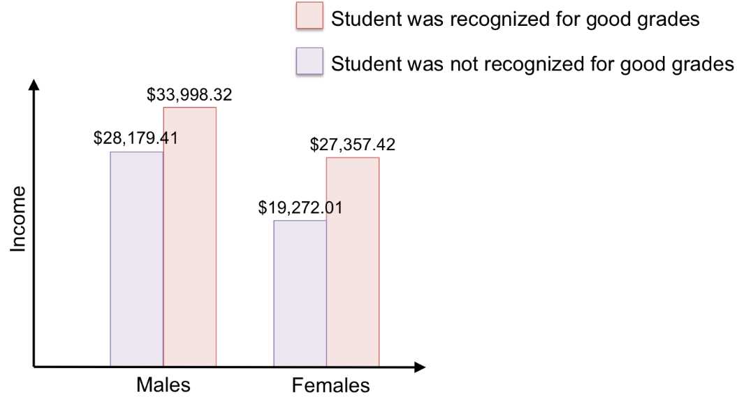
Figure 40: This bar graph visualizes the mean income for each group. Now we can see the interaction between gender and grades more clearly: females had a larger difference in income due to grades than did males.

Additional ANOVA information

Make sure you understand the data before accepting the results of ANOVA. For example, does your data have outliers? These can result in a Type I error (rejecting the null hypothesis when it is, in fact, true) or Type II error (failing to reject the null when there is, in fact, a significant difference) by pulling the mean toward it, so that the mean is not a good measure of center.

For ANOVA to have accurate results, the dependent variable should be normally distributed, have roughly equal sample sizes, and have roughly equal variances. Of course, this is not often the case, but there are methods to transform your data so that it no longer violates these assumptions. These additional tests and transformation methods are beyond the scope of our material, but there is a plethora of information online that describes what you can do for your data’s situation.

In the next lesson, you’ll learn statistical tests for tabulated data—determining whether or not frequencies (rather than specific values) differ significantly from what was expected.