Enhancing Cubes with MDX

---

One of the benefits of using an Analysis Services database for reporting and analysis (instead of using a relational database) is the ability to store business logic as calculations directly in the cube. That way, you can ensure that a particular business metric is calculated the same way every time, no matter who is asking to view the metric and no matter what skill level they have. To store business logic in the cube, you use MDX, which is the abbreviation for multidimensional expression language. MDX is also a query language that presentation layer tools use to retrieve data from a cube.

I’ll begin this chapter by explaining how to add basic calculations to the cube. Users can access these calculations just like any other measure.  The calculation designer includes several tools to help you create calculations, ranging from finding the right names of objects to selecting functions or templates for building calculations. In this chapter, you learn how to create simple calculations and how to use expressions to change the appearance of calculation results, so that users can tell at a glance whether a number is above or below a specified threshold. In addition, this chapter shows you how to use expressions to add custom members and named sets to a dimension. You will also learn about the more specialized types of expressions for key performance indicators to track progress towards goals and for actions to add interactivity to cube browsing.

Calculated Members

To create a calculated member, open the Calculation tab of the Cube Designer in SSDT and click New Calculated Member in the toolbar, the fifth button from the left. The Form View asks for the information that we need based on the type of calculation we’re creating. For a calculated member, you need to supply a name and an expression, and set the Visible property at minimum, as shown in Figure 65. The name needs to be enclosed in braces if it has spaces in it or starts with a numeric value, and the expression must be a valid MDX expression.

65. New Calculated Member

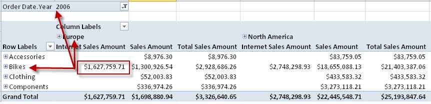
In this example, a simple addition operation combines the results of evaluating two measures, Internet Sales Amount and Sales Amount. For each cell intersection of rows and columns in a query, Analysis Services evaluates each portion of the expression individually and adds the results. That is, Internet Sales Amount is evaluated in the context of the dimensions on the current row, the current column, and the current filter, as shown in Figure 66, and the same is true for Sales Amount. Then, Analysis Services adds the results to produce the value that is displayed for Total Sales Amount having the same combination of row, column, and filter members.

66. New Calculated Member

Calculated Member Properties

A calculation also has several properties, many of which are similar to measures:

• Format String. Just as you can set a format string for a measure, you can select a built-in string or type in a custom string for a calculated member.
• Visible. Rather than try to build one complex calculation, it’s usually better for troubleshooting purposes to break it down into separate components that you hide by setting this property to False. You can then use the individual calculated members in the calculated member that is visible.
• Non-Empty Behavior. For this property, you specify one or more measures that Analysis Services should evaluate to determine whether the calculated member is empty. If you select multiple measures, all measures must be empty for Analysis Services to consider the calculated member to be empty also. On the other hand, if you do not configure this property, Analysis Services evaluates the calculated member to determine if it’s empty, which may increase query response time.
• Associated Measure Group. If you select a measure group, the calculated member will appear in the measure group’s folder in the metadata tree. Otherwise, it is displayed in a separate section of the metadata tree along with other unassociated calculated members.
• Display Folder. Another option for organizing calculated members is to use display folders. You can select an existing folder in the drop-down list or type the name of a new folder to create it.
• Color Expressions. You can define expressions to determine what font or cell color to display in the presentation tool when Analysis Services evaluates the calculated member.
• Font Expressions. You can also define expressions to determine the font name, size, or properties when the calculated member is displayed in the presentation tool.

Note: Presentation tools vary in their support of color and font expressions. Be sure to test a calculated member in each presentation tool that you intend to use and set user expectations accordingly.

Each calculated member becomes part of the cube’s MDX script. The MDX script is a set of commands and expressions that represent all of the calculations for the entire cube, including the named sets and key performance indicators that I explain later in this chapter. Using the MDX script, you can not only create calculations to coexist with the measures that represent aggregated values from the fact table, but you can also design some very complex behavior into the cube, such as changing values at particular cell intersections. However, working with the MDX script extensively requires a deep understanding of MDX and is beyond the scope of this book.

Tip: To learn more about MDX, see Stairway to MDX, an online tutorial. You can learn about working with MDX script at MDX Scripting Fundamentals at MSDN.

Calculation Tools

To help you build an MDX expression, the Calculation Designer includes several tools:

• Metadata
• Functions
• Templates

In the bottom left corner of the Calculation Designer is the Calculation Tools pane, as shown in Figure 67. The first tab of this pane displays Metadata, which contains the tree structure of the cube and its dimensions. At the top of the tree is the list of measures organized by measure group in addition to calculated members. Dimensions appear below the measures. In the metadata tree, you can access any type of object—the dimension itself, a hierarchy, a level of a hierarchy, or an individual dimension member.

67. Metadata in Calculation Tools Pane

To use the metadata tree, right-click the object to add to your expression, and click Copy. Next, right-click in the Expression box, and click Paste. You can type any mathematical operators that you need in the expression, and then continue selecting items from the metadata tree.

The Functions tab in the Calculation Tools pane contains several folders, which organize MDX functions by category. Figure 68 shows some of the navigation functions, which are very commonly used in MDX when you have hierarchies and want to do comparisons over time or percentage of total calculations.

68. Functions in Calculation Tools Pane

It’s important to understand what object type a function returns so that you can use it properly in an expression. For example, the Children function returns a set of members. Let’s put this in context by looking at the Categories hierarchy, shown in Figure 69.

69. Dimension Members in a User-Defined Hierarchy

At the top of the hierarchy is the All member, which is the parent of the members that exist on the level below: Accessories, Bikes, Clothing, and Components. You can use the Parent function with any of these members to return that All member, like this:

Likewise, you can use the Children function to get the set of members below a specified member. When you use this function with the Bikes member, the result is a set containing the Mountain Bikes, Road Bikes, and Touring Bikes members:

You can also use navigation functions to move forward and backward along the same level. For example, the NextMember function returns Road Bikes:

Likewise, using the PrevMember function with Touring Bikes also returns Road Bikes. It’s more common to use NextMember and PrevMember functions with a date dimension, but the functions work with any type of dimension. To summarize, an expression for calculated members consists of references to measures or members by using a direct reference (such as [Product].[Categories].[Mountain Bikes]) or a function to get a relative reference (such as [Product].[Categories].[Accessories].Parent). You can also perform mathematical operations on these references.

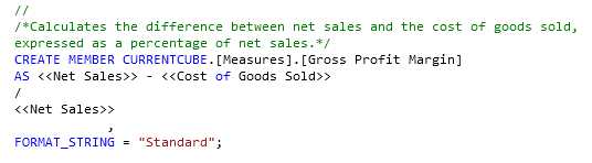
The third tab in the Calculation Tools pane is Templates. This tab provides sample expressions that you can use for many common types of calculations, as shown in Figure 70. For example, in a sales cube, you might have a calculated measure for gross profit margin. To use the template, you must first switch to Script View by using the twelfth button on the toolbar. Position the pointer below existing expressions, right-click the template, and then click Add To Template.

70. Templates for Expressions

Unlike selecting an object from the metadata tree, the template adds the complete script command to create a calculation as shown in Figure 71. The expression itself contains tokens that we need to replace with actual references from our cube. You can do that in Script View or you can toggle back to Form View (the eleventh button in the toolbar).

71. Templates for Expressions

Either way, the completed expression requires the sales amount and cost measures. In addition, you must add parentheses to the numerator expression to get the right order of operations and change the format string. That is, you must subtract cost from sales to get the margin before performing the division operation, like this:

Tuple Expressions

A common way to use navigation functions is to retrieve values for a different time period. For example, to retrieve sales for a previous period, you can combine the sales amount measure with the PrevMember function in conjunction with a date hierarchy like this:

This type of expression is known as a tuple expression. It is a coordinate that tells Analysis Services where to find information in the cube. A tuple can contain members only, which is why it’s important to know what a function returns. Because PrevMember returns a member, it’s valid for the tuple expression in the previous example.

By using a navigation function in a tuple expression, you can reposition Analysis Services away from a current member to a different member by moving forward or backward in the same level or up or down within a hierarchy. For example, in Figure 72, the Previous Period Sales Amount (based on the tuple expression defined previously), you can see the value for 2006 matches the Sales Amount value for 2005, which is the previous member on the Year level of the Year user-defined hierarchy of the Order Date dimension. Similarly, the Previous Period Sales Amount value for Q2 2006 is the Sales Amount value for Q1 2006, the previous member on the Quarter level of the hierarchy. The same is true at the month level, where the May 2006 value for Previous Period Sales Amount matches the April 2006 value for Sales Amount.

72. Effect of PrevMember function in Tuple Expression

Color and Font Expressions

Calculated members have color and font properties that are not available for measures. These color and font properties can be based on expressions, and are configured at the bottom of the Form View. However, if you know the correct syntax, you can add these expressions directly to the MDX script.

In Form View, expand the applicable section. For example, in the Color Expressions, you have the option to configure Fore Color to set the font color or Back Color to set the fill color of the cell containing a value. In the Font Expressions, you can set Font Name or Font Size. You can also set Font Flags when you want to control whether to display a value using bold or italic font styling.

Typically, you use conditional expressions for colors and fonts. A conditional expression uses the IIF function, which has three arguments. The first argument is a Boolean expression that must resolve as true or false. Usually you compare a value to a threshold here. The second argument is the value returned by the function when the Boolean expression is true, while the third argument is the value returned when the Boolean expression is false, like this:

Tip: You can use the color or font picker that is displayed to the right of the expression box to set the appropriate code in your expression. For example, you can select the color red in the picker and the value 255 appears in your expression along with a commented string, /*Red*/, as a reminder of the value’s meaning..

You should then test the result in the presentation tools that users will have, such as Microsoft Excel, as shown in Figure 73. Here, you can see the red font is displayed only wherever the gross profit margin is less than 10%.

73. Conditional Color Expression

Custom Members

Sometimes you need to create calculations that affect how measures get computed, but are not themselves measures. These are calculated members that are part of a dimension, and are also known as custom members. Let’s say that you want to support analysis of one product category relative to all other product categories. You can create a calculated member to include a total of all product categories except for Bikes. When you create a calculated member, as shown in Figure 74, you assign a name for the member that is unique within the parent hierarchy and define its parent member.

74. Name and Parent Properties for Calculated Member

After that, you define the expression for the calculated member. In this example, the calculated member’s expression uses the Aggregate function, but any function for aggregation is permissible here. That is, you can use Sum, Avg, Min, Max, DistinctCount, or Count instead.

By using the Aggregate function in the expression, you can ensure the correct values are computed for any measure that you use in a tuple expression with the calculated member. Some measures are additive, like sales and costs, while other measures are non-additive, like Gross Profit Margin. With non-additive measures, Analysis Services must sum the component parts of the expression first. With Gross Profit Margin, it needs to sum the numerator separately from the denominator, and then perform the division operation last. The Aggregate function ensures the correct order of operations, as shown in Figure 75.

75. Aggregate Function Results

The Aggregation function, like the other aggregation functions, requires a set as its first argument. A set is a collection of members from the same dimension and hierarchy. Notice that in the previous expression, the set is enclosed in braces and consists of specific members—Accessories, Clothing, and Components. In other words, the set definition explicitly lists every member of the Category hierarchy except Bikes and the All member.

Because the cube often has different types of measures, it is likely that you will need to use a conditional expression to define the format string. A CASE statement might be easier to read than a nested IIF function when there are multiple possible conditions, like this:

You can switch to Script View to more easily work with a complex conditional expression. To do this, click the twelfth button on the Calculation Designer toolbar. Another property that you might need to set in Script View is Language. Sometimes Excel or other presentation layer tools are unable to properly interpret a format string, so the language property is used to give it a hint. The complete calculated member definition in Script View looks like this:

Tip: The language identifier for United States English is 1033. If you need to use a different language identifier, refer to http://msdn.microsoft.com/en-us/goglobal/bb964664.aspx to locate the correct value.

Named Sets

You can also use the Calculation Designer to develop named sets. A named set is a special type of calculation that returns a collection of dimension members, rather than a specific value like a calculated measure. You can create a named set by defining a list of members as described in the previous example, or you can use a set function to generate a set at query time. For example, you can use the TopCount function to produce a set of the three products that have the highest sales, like this:

The first argument of the TopCount function requires a set. In this case, the expression for the first argument uses the Members function to get all the members that exist on the Product level of the Product hierarchy of the Product dimension. The second argument specifies how many members to include in the final set. The third argument specifies the measure for which Analysis Services needs to perform a descending sort of the members. In other words, this function takes the set of products, finds the total sales amount for each of them, sorts the products in descending order, and then returns the first three members of the resulting set.

When you create a named set, you specify whether you want the contents of the named set to remain constant, or the contents to change based on the context of the current query. In the Additional Properties section of the form view for a named set, select Static for a constant set or Dynamic for a set that adjusts to the query context in the Type drop-down. Figure 76 shows the effect of changing the year filter on each type of named set.

76. Static versus Dynamic Named Sets

On the left side of Figure 76, the pivot tables display a static named set while the pivot tables on the right side of the figure display a dynamic named set. The pivot tables on the top row are identical because no filters are applied to the static and dynamic pivot tables. They include the same top three products and the same values. However, the bottom row illustrates the difference between static and dynamic named sets when a filter, such as Q1 2008, is applied. On the left, the static named set includes the same three products that are displayed in the unfiltered pivot table above it, but the values in the Total Sales Amount column are applicable to Q1 2008 for those products. On the right, the dynamic named set displays a different set of three products. These three products are the top three selling products within the filtered time frame, Q1 2008, and the Total Sales Amount column displays the sales for those three products in that quarter. Thus, a static named set retains the same members regardless of filters in the query, whereas a dynamic named set includes different members depending on the query filters.

Key Performance Indicators

Another type of calculation that you can add to the cube is a key performance indicator (KPI). Technically, a KPI is not a single calculation, but a set of calculations that quantitatively describe how a value compares to a goal. In addition, a KPI includes one symbol to represent progress toward a goal and another symbol to represent the direction the KPI value is trending at a selected point in time.

Although KPIs are calculations, you use the KPI Designer to define each KPI rather than the Calculation Designer. Figure 77 shows the set of calculations for a Gross Profit Margin KPI:

77. Key Performance Indicator Form View

After you click the New KPI button in the toolbar, you define a KPI with four separate expressions: value, goal, status, and trend. Let’s look at each of them separately.

• Value. This expression represents the value to evaluate against a goal. It represents the current state of some metric. For example, to monitor gross profit margin, the value expression can simply be the measure already created for Gross Profit Margin. If the measure did not exist, you could use the expression to calculate gross profit margin here, although for troubleshooting purposes it’s better to create the calculated measure first in the Calculation Designer and then reference it in the Value expression in the KPI Designer.
• Goal. This expression is the target against which the value expression is compared. The goal could be an expression or a fixed value. In the previous example, the goal is to achieve a one percent increase in gross profit margin from the previous year. The expression to define this goal uses a tuple to retrieve the Gross Margin Percent for the same time period in the previous year and multiple it by 1.01 to get the target value.
• Status. You use the status expression to quantify how close the value is to the goal and to express the result using a range from -1 to 1. The expression should return -1 when the goal is not achieved, 0 when the value is moving toward the goal but not meeting expectations, and 1 when the value is close to the goal, at the goal, or exceeding the goal. Business requirements determine where the boundaries between -1, 0, and 1 exist. For this example, let’s say that a value of 1 is possible only when the value is within 85 percent of the goal. Otherwise, the status is 0, unless the value is below 50 percent of the goal, in which case the status returns -1. As part of the status definition, you also choose an image to associate with the status results. You can later create a dashboard constructed of KPIs (using Excel or PerformancePoint Services in SharePoint, for example) that tell you at a glance whether goals are being met.
• Trend. The trend expression compares a value in one time period to a previous period. It’s up to you to determine whether that time period is the previous period, a year-over-year period, or a moving average type of trend. As with status, you define the expression to return a value between -1 and 1. A -1 value is a negative trend that is displayed as an arrow pointing downward, whereas a 1 value is a positive trend that displays an arrow pointing upward. In the previous example, the trend expression performs a simple comparison of the current period to the previous period.

Unlike the Calculation Designer, you can use a browser built into the KPI Designer to check the results of your KPI definition. You must first deploy your project to save the KPI definition, and then click the Browser View button (the tenth button on the KPI Designer toolbar). In the browser, you can define filters to observe the changes to the KPI results, as shown in Figure 78. To view status and trend values that depend on time comparisons, you must include a Date dimension in the filter.

78. Key Performance Indicator Browser View

Tip: After changing a dimension filter in the browser view, click anywhere in the Display Structure area to apply the filter and update the KPI values.

Actions

Another way to enhance a cube is to define an action on the Actions tab of the Cube Designer. An action is a feature of Analysis Services that allows the user to initiate a process in the context of a current query, such as opening a webpage or launching a report. You can add any of three types of actions to a cube: a standard action, a drillthrough action, or a reporting action.

Regardless of its type, an action has a target, which is the object in the cube that the user clicks to trigger the action. A target can be a member of an attribute, hierarchy, level, or dimension; a cell, hierarchy, or level; or even the cube itself. When a user explores the cube, the client application displays available actions associated with a target. The steps to display or launch an action depend on the client application. For example, Excel displays available actions when you right-click a target, such as Mountain Bikes, as shown in Figure 79. In this case, the action is assigned a target type of attribute members and a target object of Product.Subcategory is displayed in Excel. In the submenu, click Additional Actions to view the available actions, such as “Search for Mountain Bikes” in this example.

79. Action Visible in Excel

Note: Before adding actions to your cube, be sure the client application supports this feature

Standard Action

A standard action is an action that returns data or launches another application based on the selected target. When you define an action, you specify an MDX expression that resolves as a string that the action provides to another application for execution. You also assign one of the following action types to your action:

• Dataset. This type of action returns a multidimensional dataset (also known as a Cellset object) to the client application after resolving a string containing an MDX statement, which executes using an Analysis Services OLE DB provider, ADOMD.NET, or XML for Analysis.
• Proprietary. This type of action performs a task defined by the client application, which is also responsible for interpreting the string expression.
• Rowset. This type of action returns a rowset to the client application after resolving a string expression as a multidimensional or relational query. It differs from the dataset action type because it can use any OLE DB-compliant data source.
• Statement. This type of action executes an OLE DB command after resolving a string as an MDX statement, such as a CREATE SUBCUBE statement. The result returned by the action is the status of statement execution, success or failure.
• URL. This type of action opens a webpage in a browser window after resolving a string as a URL.

Note: Most of these action types require the use of a custom application to interpret and execute the action and to use the results of execution in some way. If you are using Excel or PerformancePoint Services, only the URL action is supported.

Because the URL action type is the most commonly used of the available action types, let’s consider an example in which the action must open a webpage that displays Bing search results for a selected product subcategory. To create the action, click New Action (the fifth button in the toolbar) and assign a name. In this case, the target Type is Attribute Members and the Target Object is Product.Subcategory. For this action, you create an Action Expression using an MDX expression that concatenates static text and the name of the selected member like this:

You can also configure other settings for an action by expanding the Additional Properties section for the action:

• Invocation. You specify how the action occurs. If the user triggers the action, such as a URL action, this setting should be Interactive. You can also choose Batch to run the action as part of a batch operation or On Open to run it when the user opens the cube.
• Application. Here you type the name of the application to run the action as a recommendation to the client application from which the action is invoked. It is not a required property.
• Description. This property is also optional and is simply used as metadata to document the action.
• Caption. The client application displays the caption that you provide for this property. You can use static text or dynamically generate the caption by using an MDX expression. For example, you could create a custom caption for the URL action to display a string containing the name of a selected attribute member such as “Mountain Bikes” by using the following expression:

• Caption is MDX. The default value for this property is False. If you use an MDX expression for the Caption property, be sure to change this property to True.

Drillthrough Action

You add a drillthrough action to allow users to see the underlying detail data associated with a selected cell. To create the action, click New Drillthrough Action (the sixth button in the toolbar), assign a name, and select a specific measure group or all measure groups as the action target. In the Drillthrough Columns section, you select one or more combinations of dimensions and attributes to return in the drillthrough results, as shown in Figure 80.

80. Drillthrough Columns Definition for Drillthrough Action

You can configure additional properties like those available for a standard action, as well as the following properties specific to the drillthrough action:

• Default. Leave this value as False. It is available as a property to support backward compatibility when the client application executes a DRILLTHROUGH statement.
• Maximum Rows. You can specify a limit on the number of rows that Analysis Services returns when performing the drillthrough action.

In the client application, you invoke the drillthrough action from a cell containing a measure in the measure group specified as the action target. Figure 81 shows a portion of the data returned by a drillthrough action in Excel.

81. Drllthrough Results

Reporting Action

When a user launches a reporting action, the current context of the user’s selection can pass to a report hosted in Reporting Services as one or more parameters. The reporting action requires you to specify a target type and target object just like a standard action. You also specify the following report server properties:

• Server name. Here you provide the URL for the report server’s web service. This value is typically http://<servername>>/reportserver, where <servername> is the name of the computer hosting Reporting Services for a native mode installation, or http://<servername>/<site> for a SharePoint integrated mode installation, where <servername> is the SharePoint server name and <site> is the name of the site containing the document library for reports.
• Report path. The report path is the folder or path of folders containing the report and the name of the report to execute. For example, to launch a report called Total Sales by Territory in the Sales folder on a native-mode report server, you define the following report path: /Sales/Total Sales by Territory.
• Report format. You can launch the report in the default web browser by selecting the HTML3 or HTML5 options, or open the report in Adobe Reader or Excel by selecting the PDF or Excel options, respectively.

If the report contains parameters, you can provide static text or dynamic MDX expressions to configure parameter values for report execution. You type the parameter name as it appears in the report definition language (RDL) file and provide an expression that resolves to a value that is valid for that parameter, as shown in Figure 82.

82. Parameter Definition for Reporting Action

Writeback

Writeback is one of the less commonly used features of Analysis Services for two reasons. First, it requires a client application that supports it. Second, writeback is used by a relatively small number of users who need to do planning, budgeting, or forecasting, as compared to the number of users performing analysis only. In fact, the most common use of writeback in Analysis Services is in financial analytics, whether working on budgets by department or forecasting revenues and expenses. Before users commit to a final budget or forecast, they might go through several iterations of planning and can use writeback to support that process.

Note: In this section, I review the concepts for cell writeback and dimension writeback. To learn more about writeback, see Building a Writeback Application with Analysis Services.

Cell Writeback

Data normally becomes part of a cube when events occur that we want to track, such as sales or general ledger entries. However, with writeback, users can update the cube with values that they anticipate might occur, and can use the aggregation capabilities of Analysis Services to review the impact of these updates. To facilitate this activity, a client application that supports writeback is required to update a cell. In other words, writeback activity requires an update to fact data. To add data to the cube to describe what you expect or would like to see happen, you can use writeback to update values in a measure group at the intersection of selected dimension members. Typically, data captured for the writeback process is at a high-level, such as a quarter, and the Analysis Services database must contain instructions for allocating to leaf-level members like days.

Analysis Services stores the writeback data in a separate ROLAP partition, regardless of the cube storage mode (as described in Chapter 4, “Developing cubes”).  In fact, the writeback process updates a relational table and then performs an incremental process of the MOLAP partition to bring it up-to-date to match the source. Any subsequent queries to the cube return data from the MOLAP partition only. The cost of this incremental update is small compared to the impact of ROLAP queries.

To implement cell writeback, you create a writeback partition for a measure group, which can use MOLAP or ROLAP storage. As a user adds or changes values in the cube, the values stay in memory for the user’s current session and no one else can see those values. That way, a user can test the impact of changes made before finalizing the input. When finished, a COMMIT command in the writeback application recalculates user input as weighted values to leaf-level cells if the input was at higher levels. After that, T-SQL Insert statements are executed to add corresponding records to the writeback partition. If the partition uses MOLAP storage, Analysis Services performs an incremental update (as described in Chapter 6, “Managing Analysis Services databases”) to bring the cube up-to-date for faster performance.

Note: You can use cell writeback in any edition of Analysis Services.

Dimension Writeback

You can implement dimension writeback when you want to give users the ability to add new members to the dimension without requiring them to add it to the source application. However, you must have a client tool that supports dimension writeback. You can also use security to control who can use this feature, as explained in Chapter 6.

Dimension writeback is helpful when a source application is not available to maintain the members, such as a Scenario dimension. As an example, you might have a dimension like this in the data warehouse for which you preload it with members but don’t have a regular extract, transform, and load process to continually add members over time. In the AdventureWorksDW sample database, the DimScenario table has only three members to start: Actual, Budget, and Forecast.

To implement dimension writeback, you need to modify the dimension design. Specifically, you change the WriteEnabled property from its default value of False to True, and then deploy the change. If users are working with an application that supports dimension writeback, they can then add new members as needed. If you have multiple versions of budgets or forecasts that you want to keep separate during the planning process, you can also use dimension writeback to create a name used to track each version. For example, in a Scenario dimension, each member is either associated with actual data or a specific version of a budget or forecast, such as Budget v1 or Forecast v2.3.

When a user adds a new member with dimension writeback, Analysis Services updates the relational source immediately. For this reason, you can use dimension writeback only with a dimension that has a single table or an updateable view as its source. An incremental update (as described in Chapter 6) then gets the data from the relational source to update the Analysis Services database, and any subsequent queries to get dimension metadata include the new member. There is no separate storage of dimension members added in this way.

Note: You can only use dimension writeback in the Enterprise or Business Intelligence editions of Analysis Services