Developing Cubes

---

Generally, I prefer to build most, if not all, dimensions prior to developing cubes, but it’s also possible to generate skeleton dimension objects when you use the Cube Wizard. As I explain in this chapter, you use the wizard to select the tables that become measure groups in the cube and identify the dimensions to associate with the cube. After completing the wizard, you configure properties for the measures and adjust the relationships between dimensions and measure groups, if necessary. As part of the cube development process, you can also configure partitions and aggregations to manage storage and query performance. Optionally, you can add perspectives to provide alternate views of the cube and translations to support multiple languages.

Cube Wizard

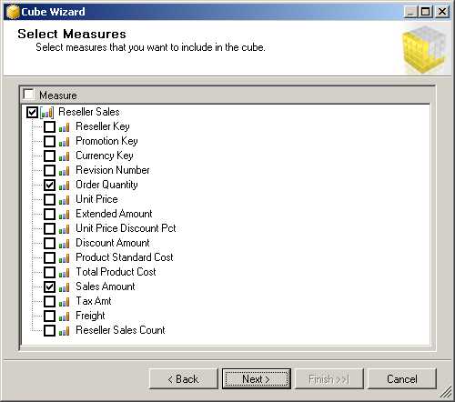
The Cube Wizard provides a series of pages to jumpstart the development of a cube. To start the Cube Wizard, right-click the Cubes folder in Solution Explorer. On the Select Creation Method page of the wizard, keep the default selection, Use Existing Tables. Just like the Dimension Wizard, the Cube Wizard offers other options to use when you want to generate tables to match specified requirements. On the Select Measure Group Tables page, shown in Figure 38, all tables in the DSV are visible and you choose those you want to use as a measure group table. Normally, a measure group table is the same as a fact table in a star schema, but that term is not used here because you can use data from other structures. In general, a measure group table is a table containing numeric values that users want to analyze and also has foreign key relationships to the dimension tables in the DSV.

38. Select Measure Group Tables Page of Cube Wizard

Tip: If you’re not sure which tables to select, click the Suggest button. The wizard examines the relationships between tables in the DSV, and proposes tables that meet the general characteristics of a fact table. This feature is useful for people who are not professional business intelligence developers but want to build a cube.

After selecting the measure group table, you see a list of all the columns in each table that have a numeric data type on the next page of the wizard, as shown in Figure 39. Some columns might not be measures, but are instead keys to dimensions, so be sure to review the list before selecting all items. Furthermore, you are not required to add all measures in a table to your cube.

39. Select Measures Page of Cube Wizard

The next page of the wizard displays dimensions that already exist in the database, as shown in Figure 40. That is, the list includes the dimensions currently visible in the Solution Explorer. You can select some or all dimensions to add to the cube.

40. Select Existing Dimensions Page of Cube Wizard

Note: If the wizard detects that a dimension could be created from the measure group table, you will see another page in the wizard before it finishes. That’s an advanced design for many-to-many relationships that is not covered in this book. If you are not familiar with handling many-to-many relationships, clear the selections on this page. To learn more about many-to-many relationships, see The Many-to-Many Revolution 2.0.

After you finish the Cube Wizard, you see the results in the Cube Designer, shown in Figure 41. The Cube Designer has many different tabs, several of which will be explored in this chapter, and others that will be explored in Chapter 5, “Enhancing cubes with MDX,” and Chapter 6, “Managing Analysis Services databases.” The first tab is for working with the cube structure. In the upper left corner, you see all the measures that you added to the cube thus far. By default, these measures appear in a tree view. If you have multiple measure groups in the cube, then you see each set of measures organized below its respective measure group.

41. Cube Structure Tab of Cube Designer

Measures

The first task to perform after building a cube is to review the properties for each measure and adjust the settings where appropriate. You should especially take care to select the appropriate aggregate function. If you later decide to add more measures to the cube, you can easily add a single measure or add multiple measures by adding a new measure group.

Measure Properties

At minimum, you should review the following properties, as shown in Figure 42: Name, FormatString, Visible, DisplayFolder, and AggregateFunction.

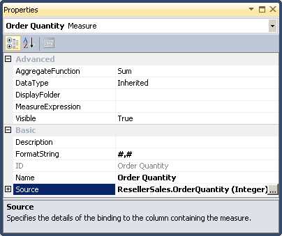
42. Measure Properties

The first thing to check for each measure is its Name property. Make sure the name appears correctly and is unambiguous for users. Measure names must be unique across all measure groups in the cube.

Next, set the FormatString property for each measure to make it easier to read the values when you test the cube in a cube browser such as Excel. You can assign a built-in format string such as Currency or Percent, or you can use a custom formatting string just as you can in Excel.

You can also choose to hide a measure by changing its Visible property to False. If you do this, the measure continues to be available for use in calculations, but anyone browsing the cube cannot see the measure.

If a measure group contains a long list of measures, you can organize them into groups by specifying a DisplayFolder value. The first time you reference a folder, you have to type in the name directly. Afterwards, the folder is available in a drop-down list so that you can assign it to other measures.

Last, review the most important property of all, AggregateFunction. The default is Sum, which instructs Analysis Services to add up each record in the fact table by dimension when returning results for a query. In the next section, I explain each of the available aggregate functions.

Aggregate Functions

There are several different types of aggregate functions available:

• Sum. The most commonly used aggregate function is the Sum function. When you use the function in a query, a list of dimension members is displayed in rows or columns (or both) and the measure is displayed at the intersection. When a dimension member is either the All level or a level in a user hierarchy that has children, the value of the measure is the sum of the children’s values for the member that you see on a particular row, as shown in Figure 43. In other words, the value for Q1 2006 is the sum of the values for Jan 2006, Feb 2006, and Mar 2006. Likewise, the value for 2006 is the sum of the values for Q1 2006, Q2 2006, Q3 3006, and Q4 2006.

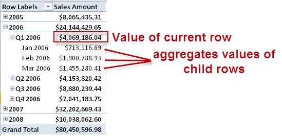
43. Aggregating Measures by Dimension Members

• Count. This is another common function. You use it to get a count of the non-empty rows in the fact table associated with the children of the current dimension member.
• Minimum, Maximum. You use these functions to find the minimum or maximum values of a member’s children, although these are less commonly used functions.
• DistinctCount. This function returns the number of unique members in a dimension that are found in a fact table. When you assign a distinct count function to a measure, it gets placed in a separate measure group to optimize performance. For the best performance, use only integer values for distinct count.
• None. When you have measures that are calculations that cannot be decomposed for some reason, such as when you have a percentage value that you want to include in a cube for use in other calculations, you can prevent aggregation for that measure by setting the Aggregate function to None.

There are several aggregate functions that are considered semi-additive. When you use a semi-additive aggregate function, the measure aggregates by using the Sum function as long as the current dimension is not the Date dimension. Within the Date dimension, the aggregation behavior depends on which semi-additive function you assigned to the measure:

• ByAccount. When you use this aggregate function, your cube must also include a dimension with the Account type and set the attribute types correctly to correctly identify accounts as Assets, Liabilities, Revenue, and Expenses, for example. With this aggregate function, the fact table values are added up properly by time according to the type of account that is displayed. For more information, see Add Account Intelligence to a Dimension.
• AverageOfChildren. As an example, if the current dimension member is a member of the quarter level of a calendar year hierarchy such as Q2 2008, Analysis Services uses this aggregate function to sum up its three months’ values (April 2008, May 2008, and June 2008), and divide the result by 3.
• FirstChild, LastChild. These aggregate functions are useful for a snapshot measure, such as an inventory count for which you load the fact table with a balance on the first day or last day of a month. Then, Analysis Services responds to a query by month with the value on the first or last day, whereas it returns the value for the first or last month for a query by quarter.
• FirstNonEmpty, LastNonEmpty. These functions behave much like FirstChild and LastChild. However, rather than using the first or last child explicitly, Analysis Services uses the first or last child only if it has a value. If it doesn’t, Analysis Services continues looking at each subsequent (or previous) child until it finds one that is not empty. For example, with FirstNonEmpty, Analysis Services looks at the second child, third child, and so on until it finds a child with a value. Likewise, with LastNonEmpty, it looks at the next to last child, the one before that, and the one before that, and so on.

Note: It’s important to know that the semi-additive functions are available only in Enterprise and Business Intelligence editions for production. You can also use Developer’s Edition to create a project that you later deploy to a production server. An exception is the LastChild function, which is available in all editions.

Additional Measures

As you develop a cube, you might find that you need to create additional measures for your cube. As long as the measures are in the DSV, you can right-click anywhere in the Measures pane on the Cube Structure tab of the Cube Designer, and select one of the following options:

• New Measure. Use this option to add a single measure from the dialog box, as shown in Figure 44. You must also specify usage, which sets the aggregate function.

44. Addition of New Measure

• New Measure Group. With this option, you see a list of the tables currently in the DSV. When you select a table, all the columns with numeric data types are added to the cube as measures. In that case, you might need to delete several columns because it is likely that one or more dimension keys are added as part of the group.

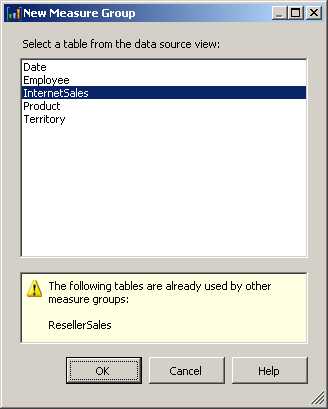
45. Addition of New Measure Group

Role-playing Dimension

A special situation arises when you have a dimension used multiple times within a cube for different purposes, known as a role-playing dimension. Before I show you what a role-playing dimension looks like, let me explain the difference between database and cube dimensions and the data structure necessary in the DSV to support a role-playing dimension in a cube.

Consider the AdventureWorksDW2012 sample database, which contains only a single date table, DimDate, for which you can create a dimension object in an Analysis Services project. Any dimension that appears in Solution Explorer is a database dimension. Not only can you associate a database dimension with one or more cubes that you add to the database, but you can also configure different properties for each instance of the dimension within a cube. However, each cube dimension continues to share common properties of the dimension at the database level.

To structure data to support a role-playing dimension, the fact table in the DSV has multiple columns with a relationship to the same dimension table, as shown in Figure 46. In this example, the Reseller Sales table (a fact table) has multiple relationships with the DateKey column in the Date table, based on the fact table’s OrderDateKey, DueDateKey, and ShipDateKey. Each column has a different meaning. The OrderDateKey stores the value for the date of sale, the DueDateKey stores the value for the promised delivery date, and the ShipDateKey is the date of shipment. Each column relates to the same date dimension because any given date has the same properties—the same month, the same quarter, the same year, day of year, and so on.

46. Multiple Foreign Key Relationships for Role-Playing Dimensions

When you add the Date dimension to the cube, the presence of the multiple relationships triggers the addition of multiple versions of the dimension to the cube as role-playing dimensions, as shown in Figure 47. You can rename each role-playing dimension if you like, or hide or delete them as determined by the users’ analysis requirements. You rename the dimension on the Cube Structure tab, because the name of a cube dimension, whether or not it’s a role-playing dimension, is a property set at the cube level and does not affect the dimension’s name at the database level.

47. Role-Playing Dimensions in Analysis Services

Dimension Usage

Much like you define foreign key relationships between fact and dimension tables in the DSV, you also define relationships between measure groups and cube dimensions on the Dimension Usage tab of the Cube Designer. In fact, if you have foreign key relationships correctly defined in the DSV, the dimension usage relationships are usually correctly defined without further intervention on your part. However, sometimes a relationship is not automatically detected, more commonly when you add measure groups to an existing cube than when you use the Cube Wizard.

You can recognize a problem in dimension usage when you see the grand total value for a measure repeat across dimension members when you expect to see separate values. For example, in Figure 48, the Sales Amount column displays separate values for each category, whereas the Internet Sales Amount column repeats the grand total value.

48. Aggregation Error Due to Missing Relationship

On the Dimension Usage tab of the Cube Designer, as shown in Figure 49, you can see that the intersection between the Product dimension and the Internet Sales measure group is empty. Dimension usage is the link between the measures in the measure group and the dimension. If the link is missing, Analysis Services is unable to aggregate fact table records by dimension member, and can only display the aggregate value for all fact table records as a whole.

49. Dimension Usage Tab of Cube Designer

To add the correct relationship, click the intersection between a dimension and a measure group, and then click the ellipsis button that is displayed. In the Define Relationship dialog box, shown in Figure 50, select Regular in the Select Relationship Type drop-down list, and then select the attribute that has a key column defined as a foreign key column in the fact table. Last, select that foreign key in the Measure Group Column drop-down list.

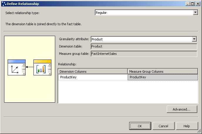
50. Dimension Usage Relationship Definition

After you deploy the project to update the cube, you can test the results by browsing the cube. With the relationship defined for dimension usage, the values for Internet Sales Amount are now displayed correctly, as shown in Figure 51.

51. Corrected Aggregation

Partitions

Analysis Services stores fact data in an object called a partition. You can use multiple partitions as a way to optimize the query experience for users and administrative tasks on the server, but you need to understand how to develop a proper partitioning strategy to achieve your goals. The main reason to partition is to manage physical storage, so it’s important to understand the different options that you have. Then you can perform the steps necessary to design a partition and to combine partitions if you later need to change the physical structure of your cube.

Partitioning Strategy

To the end user, a cube looks like a single object, but you can manage the data in a cube as separate partitions. More accurately, each measure group is in a separate partition, but you can create multiple partitions to achieve specific performance and management goals for a cube. There are three main reasons why you should consider dividing a measure group into separate partitions:

• Optimize storage. You can define different storage modes for each partition: MOLAP, HOLAP, or ROLAP. Your choice affects how and whether data is stored on disk. You can also place each physical partition on a different drive or even on different servers to distribute disk I/O operations. I explain more about MOLAP, HOLAP, and ROLAP storage modes in the next section of this chapter.
• Optimize query performance. You can also design partitions to control the contents of each partition. When a query can find all data in a single partition, it retrieves that data more quickly. But even if the data is spread across multiple partitions, the partition scans can occur in parallel and occur much faster than a scan of a single large partition. In addition, you can set different aggregation levels for each partition, which can affect the amount of extra storage required to store aggregations and also how much faster queries can run.
• Optimize processing. Often the data that you load into a cube does not change. That means you can load it once and leave it there. Processing is the mechanism that loads data into the cube, which you will learn more about in Chapter 6. If you separate data into partitions, you can restrict processing to a single small partition to load current data and leave other unchanged data in place in separate partitions. That makes processing execute more quickly. Furthermore, even if you have to process multiple partitions, you can process them in parallel and thereby reduce the overall time required to process. The amount of parallelism that you can achieve depends on the server hardware that you use for Analysis Services.

When you create a partitioning strategy, you can use different storage modes, aggregation levels, and assign a variable number of rows per partition. For example, you can have several months’ worth of data in the current year partition, twelve months in a prior year, and 5 years or 60 months in a history partition. Another benefit of this approach is the ability to maintain a moving window of data. You can easily drop off older data and add in new data without disrupting other data that you want to keep in the cube.

Storage Modes

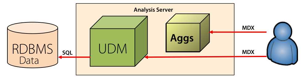
The default storage mode is called MOLAP, which is the abbreviation for Multidimensional OLAP. With MOLAP, as shown in Figure 52, all data, metadata, and aggregations are stored and managed by Analysis Services. When you process the cube, data is read from the relational source according to the rules defined in the UDM, which stands for Unified Dimensional Model. The UDM is metadata that contains all the dimension and cube definitions, describes how the data needs to be stored by Analysis Services, and contains the aggregation design, which the server processes after loading fact data to include aggregations in the data stored on the server. When a client application sends an MDX query to the server, the server responds by querying the data or aggregations in the cube.

52. MOLAP Storage

Note: MOLAP storage is an efficient way to store data in a partition. It’s highly compressed and indexed, and does not require as much space to store data as the source data.

Another storage mode is called HOLAP, which stands for Hybrid OLAP. With HOLAP, only the aggregation data and the UDM are stored on the server, but data remains in your relational database, as shown in Figure 53. When you process the cube, Analysis Services reads from the relational source and calculates the aggregations, which it then stores on the server. When a client application sends an MDX query to the server, the server responds with a result derived from aggregations if possible, which is the fastest type of query. However, if no aggregation exists to answer the query, the server uses the UDM to translate the MDX query into an SQL query, which in turn is sent to the relational source. In that case, query performance can be slower than it would be if the data were stored in MOLAP.

53. HOLAP Storage

HOLAP storage is most often used when a large relational warehouse is in place for other reasons and the majority of queries can be answered by aggregations. If the difference in performance between MOLAP and HOLAP is minimal, HOLAP might be a preferable option when you want to avoid the overhead of additional processing to create a MOLAP store of the data and the number of queries requiring the detail data is small.

The third storage mode is called ROLAP, which stands for Relational OLAP. With ROLAP, only the UDM is stored on the server while data and aggregations stay in your relational database, as shown in Figure 54. When you process the cube, no data is read from the relational source, but instead Analysis Services checks the consistency of the partition metadata during processing. Furthermore, if you design aggregations for a ROLAP partition, Analysis Services creates indexed views. As a result, there is no additional copy of data stored in Analysis Services in detail or aggregate form like there is for MOLAP or HOLAP modes.

54. ROLAP Storage

In ROLAP mode, when a client application sends an MDX query to the server, the server translates the request into SQL and returns the results from the source. Query performance is slower than it would be if the data were stored in MOLAP mode. However, the benefit of this approach is access to fresh data for real-time analysis. In MOLAP mode, the data is only as current as the last time the partition was processed.

You can also store dimension data in ROLAP storage mode. When you do this, the dimension data does not get copied to Analysis Services during processing. Instead, dimension data is retrieved only in response to a query. Analysis Services maintains a cache of dimension data that updates with each request. That cache is the first place Analysis Services looks before it issues the SQL query to the relational source. You use this option only for very large dimensions with hundreds of millions of members, which makes it a rarely used feature of Analysis Services.

Your choice of correct storage mode depends on your requirements. Larger data volumes with near-real-time data access requirements benefit from ROLAP mode. In that case, queries to your cube return data as soon as it is inserted into the relational database without the overhead of time required to process the data. On the other hand, MOLAP queries tend to be faster than ROLAP queries.

Partition Design

When you create a new partition, there are two ways that you can design it: table binding or query binding.

With table binding, you have multiple fact tables for a measure group and each fact table contains a separate set of data. For example, you might have a separate fact table for different time periods. In that case, you bind each individual table to a specific Analysis Services partition.

Partitions are not required to have common boundaries. That means one partition could have one month of data, another partition could have one year of data, and a third partition could have five years of data. Regardless, the source fact table needs to contain the data to load into the partition. There is no way to filter out data from a fact table when using the table binding method. The partition contains all the data associated with an entire table.

Tip: The problem with table binding is that changes to your fact table structure require you to manually update each partition definition to correspond. One way to insulate yourself from this problem is to bind the partitions to views instead of tables.

The other option is to use query binding. That way, you can leave all data in a single table which might be easier to manage when loading the fact table. The query for each partition includes a WHERE clause to restrict the rows that Analysis Services copies from the table to the partition during processing.

Tip: The potential problem with query binding is that you have to be very careful that no two partitions overlap. Make sure that each WHERE clause gets a unique set of rows. Analysis Services does not check for duplicate rows across partitions and if you inadvertently create this error, the data in the cube will be wrong. You should also be aware that query binding breaks the measure group’s relationship to the data source view. Consequently, if you make changes to the data source view later, those changes do not update the partition. You’ll have to do this manually. Therefore, setting up partitions should be the last step of the cube development process.

Partition Merge

You might decide to combine two or more partitions into one at some point. This process is called merging partitions. Let’s say that you have a partitioning strategy that assigns each year to a separate partition. As query patterns change, you might prefer to combine the oldest two partitions into a single partition. To do this, you can use a dialog box in SSMS to merge the partitions manually. If this is a process that you run very infrequently, this is a perfectly fine way to do this task.

If you prefer to automate the process, you can create an XMLA script in Management Studio to run the merge. You can then incorporate the script into an Integration Services package using an Execute DDL task. You can also create variables for the partition identifiers in the script so that you can reuse it to merge other partitions.

Aggregations

The key to fast query performance in Analysis Services is the addition of aggregations to each cube. Having aggregations available in the Analysis Services database is much like having summary tables in a data warehouse, except you don’t have to build or maintain the aggregations as you do with summary tables. Analysis Services does most of the work.

Aggregation Wizard

You begin the process of adding aggregations by launching the Aggregation Wizard. To do this, open the Aggregations tab of the Cube Designer and click the first toolbar button. On the Review Aggregation Usage page of the wizard, you can adjust settings to fine-tune the aggregation design process, but in most cases the default settings are adequate.

On the Specify Object Counts page of the wizard, shown in Figure 55, you can click Count to retrieve actual row counts from the tables associated with the measure group and dimension objects, or you can type an estimated count to more accurately reflect your production environment when you are working against a development database. The cube objects list includes the measure group and attributes included in a user-defined hierarchy.

The Aggregation Wizard uses the estimated count to calculate the ratio of members in an attribute relative to the fact table rows and determine whether the attribute is a candidate for aggregation. For example, because the number of members for the Group attribute is 4 and the number of records in FactResellerSales is 60,855 (when using the AdventureWorksDW2012 database as a source), there is a high probability (but no guarantee) that the Aggregation Wizard will generate at least one aggregation that includes Group. In general, if the number of attribute members is 30 percent or less than the fact table records, Analysis Services considers the attribute as a candidate for aggregation.

55. Specify Object Counts Page of Aggregation Wizard

On the next page, shown in Figure 56, you select one of the following aggregation options:

• Estimated Storage. Use this option to constrain the disk space requirements for aggregations.
• Performance Gain. Use this option to add enough aggregations to improve query speed by a specified percentage as compared to a query against a cube having no aggregations. The default is 30 percent, but you should begin with a value between 5 and 10 percent.
• Stop. Use this option to interrupt the aggregation design process by clicking the Stop button.
• Do Not Design Aggregations. Use this option or click Cancel to stop the wizard.

56. Specify Object Counts Page of Aggregation Wizard

Note: For more information, see Aggregation Design Strategy. Although the article is written for SQL Server 2005 Analysis Services, the principles remain applicable to all later versions through SQL Server 2012 Analysis Services.

On the last page of the wizard you have the option to deploy the changes and compute aggregations, or to save the aggregation design without deploying the changes to the server (in case you want to make other modifications to the database design first). By completing the wizard, you add one or more aggregation designs to your project. If you also deploy the aggregations, Analysis Services uses this aggregation design to calculate aggregations and store the results on disk.

An aggregation design is a template that Analysis Services uses to define the dimensions to include with aggregations. Although you can see the aggregation design in SSDT or the database script, you cannot see the aggregation values themselves if you use the default MOLAP storage mode for measure group partitions. However, if you use ROLAP storage, you can see the indexed views that Analysis Services uses for aggregations, such as the one shown in Figure 57. To set up ROLAP storage, click the Storage Settings link on the Partitions tab of the Cube Designer for the measure group, select Real-time ROLAP, click the Options button, and select the Enable ROLAP Aggregations check box.

57. Indexed View for ROLAP Aggregations

As you will learn later in Chapter 6, ROLAP storage keeps all data for a cube in a relational database, including the aggregations. However, MOLAP storage keeps all data on disk in a proprietary format. When a user executes a query against a measure group using MOLAP storage, Analysis Services executes a query that returns data much like you see in the indexed view. In essence, it queries the fact data and performs a group by operation on the designated attributes. However, when a measure group is using ROLAP storage, Analysis Services performs a relational query for ROLAP data. Each time you process the cube, each aggregation is updated to remain synchronized with the measure group data.

Aggregation Designer

To see how the aggregation design corresponds to the aggregation itself, let’s look at the Aggregation Designer. To open the Aggregation Designer, shown in Figure 58, click the Aggregations tab of the Cube Designer. Next, click Advanced View in the toolbar, and make your selections in the Measure Group and Aggregation Design drop-down lists.

58. Aggregation Designer

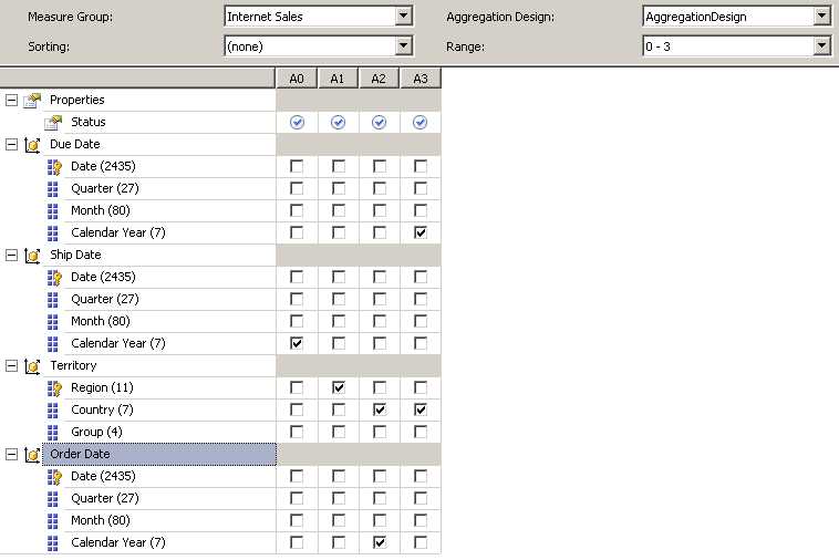
The first aggregation is labeled A0, which is the abbreviation for Aggregation 0. The check boxes in this column identify the attributes to include in the aggregation. In this case, A0 includes only the Calendar Year aggregation. The A3 aggregation, containing Calendar Year and Country, is the aggregation corresponding to the indexed view shown in Figure 57. These four aggregations are useful when user queries ask for measures by ship date calendar year, by region, by country and order date calendar year, or by due date calendar year and country. Furthermore, a query for sales by group in the Territory dimension can use the aggregation by country to derive the group values, which Analysis Services can do much faster than by adding up fact data and grouping by country at query time.

However, if a user asks for sales by region and year, Analysis Services cannot use any of these aggregations. Instead, it will have to add up the individual transactions in the fact table and group by region and year, which takes much longer for thousands of rows than the handful of rows in these aggregations. Similarly, a query for sales by country and order date quarter cannot be answered by these aggregations, nor can a query for sales by country and order date month.

Analysis Services uses an algorithm to come up with the set of aggregations that are most useful for answering queries, trying to strike a balance between storage, processing time, and query performance, but there’s no guarantee that the aggregations it creates are the aggregations that are best for user queries. Analysis Services can use any attribute to build aggregations. Essentially, it does a cost-benefit analysis to determine where it gets the most value from the presence of an aggregation as compared to calculating an aggregated value at run time.

After you use the Aggregation Wizard, or even if you choose not to use the wizard, you can add new aggregations or modify existing aggregations by using the Aggregation Designer. Let’s say that you’ve been made aware of some query performance problems. You can use SQL Server Profiler to start a trace and review the trace results to find out if aggregations are being used and to see what data is being requested. If Analysis Services can use an aggregation, you will see the event in the trace, as shown in Figure 59. You can also see which aggregation was used by matching it to the number you see in the Aggregation Designer. Furthermore, you can measure the duration of the associated Query Subcube event. If the duration is less than 500 milliseconds, the aggregation doesn’t require any change.

59. SQL Server Profiler Trace with Aggregation Hit

When you find a Query Subcube event without an aggregation but with a high duration, you can use the information in the Query Subcube verbose event to determine which attributes should be in an aggregation design. In the Text field, any attribute without a 0 next to it is a candidate. For example, in Figure 60, you can see that the attributes Subcategory, Category, Calendar Year, and Quarter are each displayed with an asterisk. Therefore, you should consider creating an aggregation for Subcategory and Quarter.

60. SQL Server Profiler Trace with Aggregation Hit

Tip: It is not necessary to create an aggregation for attributes in higher levels of the same category. That is, you do not need to create an aggregation for Year because the lower-level Quarter aggregation suffices. Similarly, the Subcategory aggregation negates the need to create a Category aggregation.

The toolbar in the Advanced view of the Aggregation Designer allows you to create a new aggregation design, either by starting with an empty aggregation design or by creating a copy of an existing design. You can do this if you don’t have an existing aggregation design on the partition accessed by the query, or you want to replace the existing aggregation design. Simply click New Aggregation Design on the toolbar to start a new design. Then you can click New Aggregation on the toolbar to add a new aggregation and select the check boxes for the lowest level attribute of a hierarchy necessary to support user queries. In the previous example, the selection includes only the Subcategory and Quarter attributes.

Usage-Based Optimization

The problem with the Aggregation Wizard is that the aggregation design process is based on the counts of dimension members relative to fact records. In practice, there’s no point in creating aggregations if they don’t help queries that are actually executing. Fortunately, you can use Usage-Based Optimization (UBO) to find out which queries are running and design aggregations to better support those queries.

To work with UBO, you first need to configure the query log on the Analysis Server. Open SQL Server Management Studio, connect to Analysis Services, right-click the server node, and click Properties. There are four properties to configure, as shown in Figure 61.

61. SQL Server Profiler Trace with Aggregation Hit

By default, the query logging mechanism is not enabled. To enable it, set the CreateQueryLogTable property to true. For the QueryLogConnectionString property, you must provide a connection string for a SQL Server database in which you want to store the log. In addition, you need to specify a sampling rate. For initial analysis of queries, you should change the QueryLogSampling value to 1 to capture every query. Lastly, you can customize the name of the table in which to store the query log data in the QueryLogTableName property. The default table name is OlapQueryLog.

Tip: When you have finished capturing log data, you can clear the connection string to discontinue logging. If you do keep the query logging active, Analysis Services deletes records from the table when you make structural changes that impact aggregation design, such as changing the number of measures in a measure group, changing the number of dimensions associated with a measure group, or changing the number of attributes defined for a dimension.

After enabling the query log, you can run standard reports or just let users browse the cube using their favorite tools for a period of time, such as a week or a month. During that time, usage information about queries is added to the query log table. This table tracks queries by database, the partition queried, and user. It also records the dataset used, the start time, and the query duration. The dataset is in a format that matches the Query Subcube Event that you see in Profiler.

When you’re ready to design aggregations based on usage, launch the Usage Based Optimization wizard. In SSDT, click the second button on the toolbar of the Aggregations tab in the Cube Designer. After you launch the wizard, you can filter the contents of the query log by date, user, or most frequent queries. If you need to filter by other values, you can execute a T-SQL script to delete rows from the query log manually.

As you step through the wizard, you can see information about the queries, such as the attributes used, the frequency of that combination of attributes in queries, and the average duration of queries. You can’t change any information here, but you can sort it and see what kind of activity has been captured. The remaining steps in the Usage Based Optimization Wizard are very similar to the steps in the Aggregation Wizard.

Perspectives

By default, all objects that you create in a cube are visible to each user, unless you apply security to dimensions, dimensions members, or cells as described in Chapter 6. When a cube contains many objects, you can simplify the cube navigation experience for the user by adding a perspective to the cube. That way, the user sees only a subset of the cube when browsing the metadata to select objects for a query, as shown in Figure 62.

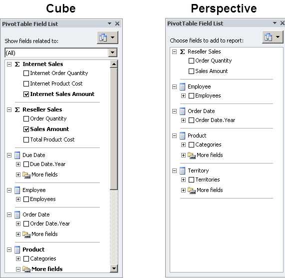
62. Browsing a Cube versus a Perspective

To create a perspective, open the Perspectives tab in the Cube Designer, and then click New Perspective on the toolbar. You can assign a name to the new perspective, and then clear or select check boxes to identify the objects to exclude or include respectively, as shown in Figure 63.

63. New Perspective

You can include any of the following object types in a perspective:

• Measure group
• Measure
• Calculation
• Key performance indicator
• Dimension
• Hierarchy
• Attribute

Note: A perspective cannot be used as a security measure. Its sole purpose is to simplify the user interface by displaying a subset of objects in a cube. To prevent users from viewing sensitive data, you must configure security as described in Chapter 6.

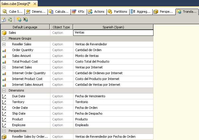
Translations

Just as you can display translations for dimensions as described in Chapter 3, “Developing dimensions,” you can also set up translations for a cube. However, there is no option to retrieve the translation from a relational source. Instead, you must manually type the translated caption for the cube, measure groups, measures, dimensions, and perspectives. To add the translations, open the Translations tab of the Cube Designer, click New Translation on the toolbar, and type the applicable caption for each object, as shown in Figure 64.

64. Translation Captions in a Cube