Matrices

---

Matrices are arguably the most important data structure used in numeric and scientific programming. The following screenshot shows you where this chapter is headed.

Figure 22: NumPy Matrices Demo

In section 3.1, you'll learn the most common ways to create and initialize NumPy matrices, and learn the differences between the two kinds of matrix data structures supported in NumPy.

In section 3.2, you'll learn how to perform matrix multiplication using the dot() function.

In section 3.3, you'll learn about the three different ways to transpose a matrix.

In section 3.4, you'll learn about the important NumPy and SciPy linalg modules, how to find the determinant of a matrix using the det() function, and what the determinant is used for.

In section 3.5, you'll learn how to create an identity matrix using the eye() function, find the inverse of a matrix using the linalg.inv() function, and correctly compare two matrices for equality using the isclose() function.

In section 3.6, you'll learn how to load values into a matrix from a text file using the loadtxt() function.

3.1 Matrix Initialization

Matrices are arguably the most significant feature of the NumPy library. NumPy supports two kinds of matrices: n-dimensional array style matrices and explicit NumPy matrices. The two kinds of matrices are mostly compatible with each other. NumPy matrices can be created in many ways, but three common techniques in many data science scenarios are using the matrix() function, the array() function, and the zeros() function.

Code Listing 8: Matrix Initialization Demo

The demo program begins by creating a matrix using the NumPy matrix() function:

ma = np.matrix([[1.0, 2.0, 3.0],
                [4.0, 5.0, 6.0]])

There are two rows, each with three columns, so the matrix has shape 2×3. Because no dtype argument was specified, each cell of the matrix holds the default float64 data type.

Next, the demo creates a 3×2 matrix using the NumPy zeros() function:

mb = np.zeros((3, 2), dtype=np.int32)

Notice the double sets of parentheses used here as opposed to the single set of parentheses used to create a simple array. Each cell of matrix mb holds a 32-bit integer. If the dtype argument had been omitted, each cell would have been the default float64 data type. As you'll see shortly, matrix mb is actually a NumPy n-dimensional array rather than a NumPy matrix. In the vast majority of programming situations, you can use either a NumPy 2-dimensional array or a NumPy matrix. The general terms matrix and matrices can refer to either a NumPy matrix or a NumPy n-dimensional array.

Next, the demo creates two additional matrices:

mc = np.array([[1.0, 2.0, 3.0], [4.0, 5.0, 6.0]])
md = np.matrix([[7.0, 8.0, 9.0]])

Matrix mc is a 2×3 n-dimensional array with the same values as explicit matrix ma. Matrix md is a 1×3 matrix. Matrices with one row are often called row matrices. Matrices with one column are called column matrices. For example:

mm = np.matrix([[7.0], [8.0], [9.0]])

Row and column matrices are not the same as simple one-dimensional arrays. You can create a column matrix from a row matrix (or vice versa) using the reshape() function, for example, mm = np.reshape(md, (3,1)). And you can make a regular array from an ndarray-style matrix using the flatten() or ravel() functions, for example:

aa = np.array([[1.0, 2.0, 3.0], [4.0, 5.0, 6.0]])  # a 2x3 ndarray matrix
arr = np.flatten(aa)  # arr is an array [1.0, 2.0, 3.0, 4.0, 5.0, 6.0] 

After displaying the contents of matrices ma, mb, and mc, the demo displays their object types:

print "ma is type " + str(type(ma))  # 'numpy.matrixlib.defmatrix.matrix'
print "mb is type " + str(type(mb))  # displays 'numpy.ndarray'
print "mc is type " + str(type(mc))  # displays 'numpy.ndarray'

To summarize, when creating a NumPy matrix, the result can be either an explicit matrix (for example, when using the matrix() function) or an ndarray (for example, when using the zeros() function). In most cases, you don't have to worry about what the object type is because the two forms of matrices are usually (but not always) compatible.

Next, the demo displays the contents of matrix ma using the program-defined show_matrix() function:

print "Contents of matrix ma using show_matrix(ma, 3, 6) are "
show_matrix(ma, 3, 6)

The second and third parameters for show_matrix() are the number of decimals to use and the width to use when displaying each cell value. In situations like this, where there are similar parameters, it's more readable to use named-parameter syntax like:

show_matrix(ma, dec=3, wid=6)

Function show_matrix() illustrates how to traverse a matrix:

def show_matrix(m, dec, wid):
  fmt = "%" + str(wid) + "." + str(dec) + "f"
  (rows, cols) = np.shape(m)
  for i in xrange(rows):
    for j in xrange(cols):
      print fmt % m[i,j],
    print ""  # end of row
  print "" # final newline

The dimensions of the matrix are determined using the NumPy shape() function, which returns a tuple with the number of rows and columns. An alternative approach is:

rows = len(m)
cols = len(m[0])

A NumPy matrix m is an array of arrays. So len(m) is the number of rows, m[0] is the first row, and len(m[0]) is the number of cells in the first row, which is the same as the number of columns (assuming all rows of m have the same number of columns).

The nested for loops iterate over the cells of the matrix from left to right, then top to bottom:

for i in xrange(rows):
  for j in xrange(cols):
    # curr cell is m[i,j]

Interestingly, NumPy allows you to access a matrix cell using either m[i,j] syntax or m[i][j] syntax. The two forms are completely equivalent. In most cases the m[i,j] form is preferred, only because it's easier to type.

Next, the demo program illustrates matrix addition:

msum = ma + mc
print "Result of ma + mc = "
print msum

Recall that both ma and mc are 2×3 matrices with values 1.0 through 6.0:

[[ 1.0  2.0  3.0]
[ 4.0  5.0  6.0]]

Not surprisingly, the result (where I've added 0s after the decimal points for readability) is:

[[ 2.0   4.0   6.0]
[ 8.0  10.0  12.0]]

However, recall that ma is an explicit NumPy matrix but mc is a NumPy ndarray. The point is that the two different types of matrices could be added together without any problems.

Next, the demo shows an unusual feature of NumPy called broadcasting:

md = np.matrix([[7.0, 8.0, 9.0]])
mx = ma + md
print "Result of ma + md is "
print mx

Matrix ma is 2×3. Matrix md is 1×3. In just about any other programming language that I'm aware of, an attempt to add these two matrices would generate some kind of error because these matrices have different shapes. However, NumPy allows the addition and returns:

[[  8.0  100.  12.0]
[ 11.0  13.0  15.0]]

NumPy essentially expands the 1×3 md matrix to a 2×3 matrix, duplicating values, so that it has the same shape as ma, and then corresponding cells can be added. Some of my colleagues think NumPy broadcasting is a wonderful, useful feature. Others feel that broadcasting is a dubious feature that encourages sloppy coding and can easily lead to program bugs.

Resources

For a discussion of the differences between NumPy matrices and arrays, see
http://www.scipy.org/scipylib/faq.html#what-is-the-difference-between-matrices-and-arrays.

For details about creating matrices using the NumPy matrix() function, see
http://docs.scipy.org/doc/numpy-1.10.1/reference/generated/numpy.matrix.html.

For details about creating ndarray style matrices using the NumPy array() function, see
http://docs.scipy.org/doc/numpy-1.10.1/user/basics.creation.html.

3.2 Matrix Multiplication

Performing matrix multiplication is a very common task in many numeric programming scenarios. The NumPy dot() function performs matrix multiplication.

The demo program in Code Listing 9 illustrates matrix multiplication using NumPy. The program then defines a custom function named my_mult(), which performs matrix multiplication using nested loops. Program execution begins with a preliminary print statement and then the demo creates a 2x3 matrix A, and a 3x2 matrix B using the NumPy matrix() function:

A = np.matrix([[1.0, 2.0, 3.0],
               [4.0, 5.0, 6.0]])

B = np.matrix([[7.0, 8.0],
               [9.0, 10.0],
               [11.0, 12.0]])

Code Listing 9: Matrix Multiplication Demo

After creating the two matrices and displaying their values, we compute their product using the NumPy dot() function and then again using the program-defined my_mult() function like so:

C = np.dot(A, B)
D = my_mult(A, B)

NumPy matrix objects can also be multiplied using the * operator, for example C = A * B, but ndarray objects must use the dot() function. In other words, the dot() function works for both types and so is preferable in most situations.

The demo concludes by displaying both results to visually verify they're the same:

Matrix multiplication is perhaps best explained by example. Matrix A has shape 2×3 and matrix B has shape 3×2. The shape of their product is 2×2:

(2 x 3) * (3 x 2) = (2 x 2)

You can imagine that the two innermost dimensions, 3 and 3 here, cancel each other out, leaving the two outermost dimensions. For example, a 5×4 matrix times a 4×7 matrix will have shape 5×7. If the two innermost dimensions are not equal, NumPy will generate a "shapes not aligned" error.

The result value at cell [x,y] is the product of the values in row x of the first matrix and column y of the second matrix. So for the demo, the result at cell [0,1] uses row 0 of matrix A = [1, 2, 3] and column 1 of matrix B = [8, 10, 12], giving (1 * 8) + (2 * 10) + (3 * 12) = 64.

The implementation of program-defined function my_mult(a, b) begins by determining the number of rows and columns in each of the two matrix parameters by using the NumPy shape() function:

def my_mult(a, b):
  (arows, acols) = np.shape(a)
  (brows, bcols) = np.shape(b)
. . .

The shape() function returns a tuple holding the number of rows and the number of columns in a matrix. You could perform an error check here to verify that the two matrices are conformable, for example, if acols != brows: print "Error!".

Once the sizes of the two input matrices are known, a result matrix with the correct shape can be initialized using the NumPy zeros() function:

result = np.zeros((arows, bcols))

Notice the use of double parentheses, which forces the zeros() function to return a matrix rather than an array. Function my_mult() then iterates over each row and each column, accumulating and storing the sum of products into each cell of the result matrix:

for i in xrange(arows):
  for j in xrange(bcols):
    for k in xrange(acols):
      result[i,j] = result[i,j] + a[i,k] * b[k,j]
return result

Notice that the program-defined matrix multiplication function is quite simple but does involve triple-nested for loops. For small matrices, the difference in performance between a program-defined method and the NumPy dot() function probably isn't significant in most scenarios. But for large matrices, the slower performance of a program-defined method would likely be noticeable and annoying.

The dot() function can be applied to NumPy one-dimensional arrays as well as matrices. For example:

>>> import numpy as np
>>> arr1 = np.array([1, 3, 5])
>>> arr2 = np.array([6, 4, 2])
>>> arr3 = np.dot(arr1, arr2)
>>> print arr3
28

In this example, the result is calculated as (1 * 6) + (3 * 4) + (5 * 2) = 6 + 12 + 10 = 28. In math terminology, this is called the dot product (hence the name of the NumPy function), the scalar product, or the inner product.

NumPy has a dedicated inner() function that works just with arrays. For example:

>>> arr4 = np.inner(arr1, arr2)
>>> print arr4
28

One possible program-defined implementation of an array dot product function is:

def my_dotprod(a1, a2):
  result = 0
  for i in xrange(len(a1)):
    result = result + a1[i] * a2[i]
  return result

The dot() function can also be applied to arrays with three or more dimensions, but this is a relatively uncommon scenario.

Resources

For additional details on the NumPy dot() function, see
http://docs.scipy.org/doc/numpy/reference/generated/numpy.dot.html.

For a table that lists the approximately 60 NumPy matrix functions, see
http://docs.scipy.org/doc/numpy-1.10.1/reference/generated/numpy.matrix.html.

For information on the NumPy ndarray data type, which includes matrices, see
http://docs.scipy.org/doc/numpy-1.10.1/reference/arrays.ndarray.html.

3.3 Matrix Transposition

A simple but common matrix operation is transposing rows and columns. The NumPy library supports three built-in ways to transpose a matrix m: the m.transpose() function, the np.transpose(m) function, and the m.T property.

Code Listing 10: Matrix Transposition Demo

The demo program begins by creating and displaying a simple 3×3 float64 matrix:

m = np.matrix([[1., 2., 3.],
               [4., 5., 6.],
               [7., 8., 9.]])

print "Matrix m = "
print m

Here, matrix m is called a square matrix because it has the same number of rows and columns. Matrix transposition works with either square or non-square matrices.

Next, the demo program creates a transposition of the matrix m using three different NumPy built-in techniques:

mt = m.transpose()
print "Transpose from m.transpose() function = "
print mt

mt = np.transpose(m)
print "Transpose from np.transpose(m) function = "
print mt

mt = m.T
print "Transpose from m.T property  = "
print mt

The first function call uses the transpose() method of the ndarray class. Notice the syntax is matrix.transpose() and there are no arguments. The second function call uses the NumPy function that accepts a matrix as its argument. The third call has no parentheses, indicating it is a property. In all three function calls, the original matrix m is not changed. If you want to change a matrix, you can use a calling pattern along the lines of m = np.transpose(m).

An immediate and obvious question is: Why are there three ways to transpose a matrix? There's no good answer. One of the strengths of open source projects like NumPy and SciPy is that they are collaborative efforts. However, this strength is offset by a certain amount of redundancy in the libraries. Basically, when you're using NumPy and SciPy you can often perform a task several ways, and frequently there's no clear best way.

The demo program concludes by calling a custom transpose function named my_transpose():

mt = my_transpose(m)

Function my_transpose() is defined:

def my_transpose(m):
  (rows, cols) = np.shape(m)
  result = np.zeros((rows, cols))
  for i in xrange(rows):
    for j in xrange(cols):
      result[j,i] = m[i,j]
  return result

There's no advantage to using program-defined my_transpose() unless you needed to customize transposition behavior in some way.

Resources

For details about the three built-in NumPy ways to transpose a matrix, see:

http://docs.scipy.org/doc/numpy-1.10.1/reference/generated/numpy.transpose.html
http://docs.scipy.org/doc/numpy-1.10.0/reference/generated/numpy.ndarray.transpose.html
http://docs.scipy.org/doc/numpy-1.10.0/reference/generated/numpy.ndarray.T.html

3.4 Matrix Determinants

The determinant of a matrix is a value that indicates whether or not the matrix has an inverse (if the determinant is 0.0, then the matrix does not have an inverse). Determinants also indicate if a set of vectors are linearly dependent and how many solutions there are to a linear system of equations. Both NumPy and SciPy have a det() function in their linalg (linear algebra) submodules.

Code Listing 11: Matrix Determinant Demo

The demo program begins by creating and displaying a 4×4 float64 matrix:

m = np.matrix([[1., 4., 2., 3.],
               [0., 1., 5., 4.],
               [1., 0., 1., 0.],
               [2., 3., 4., 1.]])

print "Matrix m = "
print m

Determinants only apply to square matrices (those with the same number of rows and columns). The simplest case (other than a 1×1 matrix with a single value) is a 2×2 matrix. Consider the 2×2 matrix in the lower left portion of the demo matrix:

1.0  2.0
3.0  4.0

The determinant of this matrix is (1.0 * 4.0) - (2.0 * 3.0) = 4.0 - 6.0 = -2.0. In words, to calculate the determinant of a 2×2 matrix, you take upper left times lower right, and subtract upper right times lower left.

A determinant of a square matrix always exists, but it can be zero. For example, consider this matrix:

3.0  2.0
6.0  4.0

The determinant would be (3.0 * 4.0) - (2.0 * 6.0) = (12.0 - 12.0) = 0. Matrices that have a determinant of zero do not have an inverse.

For 3×3 and larger matrices, the mathematical definition of the determinant is recursive. Suppose a 3×3 matrix is:

a  b  c
d  e  f
g  h  i

In this, a, b, c, etc., represent arbitrary numbers. The determinant is:

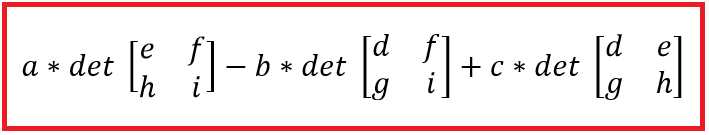
Figure 23: Definition of a 3x3 Matrix Determinant

Notice you have to extract n submatrices of size n-1 × n-1 by removing the first row and each of the n columns. Writing code from scratch to calculate the determinant of a matrix with a size larger than 3×3 is very difficult, but with NumPy and SciPy, all you have to do is call the linalg.det() function.

The demo program finds the determinant of the matrix it created like so:

d = np.linalg.det(m)
print "Determinant of m using np.linalg.det() is "
print d

Simple and easy. The NumPy linalg submodule currently has 28 functions that operate on matrices, including the det() function. The larger SciPy linalg submodule has 82 functions.

Interestingly, the SciPy linalg submodule contains a slightly different det() function. The SciPy version of det() has a parameter overwrite_a that allows the matrix to be changed during the calculation of the determinant, which improves performance. Many functions appear in both the NumPy and SciPy libraries, which is both useful and a possible source of confusion.

The demo has a program-defined function my_det() that calculates the determinant of a matrix. Let me emphasize that the program-defined function is very inefficient and is intended only to demonstrate advanced NumPy and SciPy programming techniques. The custom my_det() function shouldn't be used unless you want to demonstrate a bad way to calculate a matrix determinant.

Function my_det() uses the same calling signature as the NumPy det() function:

d = my_det(m)
print "Determinant of m using my_det() is "
print d

Function my_det() is recursive, meaning that it calls itself. The my_det() function also calls a helper function extract() defined as:

def extract(m, col):
  n = len(m)
  result = np.zeros((n-1, n-1))
  for i in xrange(1, n):
    k = 0
    for j in xrange(n):
      if j != col:
        result[i-1,k] = m[i,j]
        k += 1
  return result

Function extract(m, col) accepts an n × n matrix m and returns an n-1 × n-1 matrix from which the first row and column col have been removed. The key code in my_det() is:

for k in xrange(n):
  sign = -1
  if k % 2 == 0: sign = +1
    subm = extract(m, k)
    sum = sum + sign * m[0,k] * my_det(subm)

Each of the n sub-matrices is extracted and my_det() is called recursively. There are very few situations where recursive code is a good choice, and calculating a determinant of a matrix is not one of them. The NumPy and SciPy implementations of det() use a technique called matrix decomposition, which is complicated, but very efficient.

Resources

For details about the NumPy det() function, see
http://docs.scipy.org/doc/numpy-1.10.1/reference/generated/numpy.linalg.det.html.

For details about the SciPy det() function, see
http://docs.scipy.org/doc/scipy-0.15.1/reference/generated/scipy.linalg.det.html.

3.5 Matrix Inversion

One of the most common and important operations in numeric programming is finding the inverse of a matrix. The NumPy and SciPy linalg.inv() functions perform matrix inversion.

The demo program in Code Listing 12 illustrates matrix inversion using NumPy. As usual, at the top of the code, the program brings the NumPy library into scope and provides a convenience alias: import numpy as np.

Because the inv() function is part of the NumPy linalg (linear algebra) submodule, an alternative would be to use a from numpy import linalg statement. The demo program then defines a custom function named my_close(), which determines if two matrices are equal in the sense that all corresponding cell values are equal or nearly equal, within some small tolerance.

Program execution begins with a preliminary print statement and then the demo creates a 3×3 matrix m using the NumPy matrix() function, explicitly specifying the data type:

m = np.matrix([[3, 0, 4],
               [2, 5, 1],
               [0, 4, 5]], dtype=np.float64)

Code Listing 12: Matrix Inverse Demo

Matrix m could have been created as an n-dimensional array using the array() function:

m = np.array([[3., 0., 4.],[2., 5., 1.],[0., 4., 5.]])

After creating the matrix m and displaying its values, the inverse of the matrix is computed and displayed like so:

mi = np.linalg.inv(m)
print "The inverse of m is"
print mi

If the from numpy import linalg statement had been used at the top of the script, the inv() function could have been called as linalg.inv(m) instead. The inv() function applies only to square matrices (equal number of rows and columns) that have a determinant not equal to zero. The return value is a square matrix with the same shape as the original matrix.

Matrix inversion is one of the most technically challenging algorithms in numeric processing. Believe me, you do not want to try to write your own custom matrix inversion function, unless you are willing to spend a lot of time and effort, presumably because you need to implement some specialized behavior.

Not all matrices have an inverse. If you apply the inv() function to such a matrix, you'll get a "singular matrix" error. Therefore, you want to check first along the lines of:

d = np.linalg.det(m)
if d == 0.0:
  print "Matrix does not have an inverse"
else:
  mi = np.linalg.inv(m)

Next, the demo creates and displays a 3x3 identity matrix:

idty = np.eye(3)
print "The 3x3 identity matrix idty is"
print idty

An identity matrix is a square matrix where the cells on the diagonal from upper left to lower right contain 1.0 values, and all the other cells contain 0.0 values.

In ordinary arithmetic, the inverse of some number x is 1/x. For example, the inverse of 3 is 1/3. Notice that any number times its inverse equals 1. The identity matrix is analogous to the number 1 in ordinary arithmetic. Any matrix times its inverse equals the identity matrix.

The demo verifies the inverse is correct by multiplying the original matrix m by its inverse mi and displaying the result, which is, in fact, the identity matrix:

print "Product of mi * m is"
mim = np.dot(mi, m)
print mim

The output is somewhat difficult to read because of the print statement's default formatting:

Product of mi * m is
[[  1.00000000e+00  -1.11022302e-16   0.00000000e+00]
[  0.00000000e+00   1.00000000e+00   0.00000000e+00]
[  0.00000000e+00   1.11022302e-16   1.00000000e+00]]

If you look closely, you'll see that that main diagonal elements are 1.0 and the other cell values are very, very close to 0.0. Visual verification that two matrices (the product of the original matrix times its inverse, and the identity matrix) are equal is fine in simple scenarios, but in many situations a programmatic approach is better. The demo compares the matrix times its inverse (mim) and the identity matrix in two ways:

b1 = np.allclose(mim, idty)
print "Comparing mi * m with idty using np.allclose() gives"
print str(b1)

b2 = my_close(mim, idty, 1.0e-4)
print "Comparing mi * m with idty using my_close() gives"
print str(b2)

In general, it's a bad idea to compare two matrices that hold floating-point values for exact equality because floating-point values have some storage limit and therefore are sometimes only approximations to their true values. For example:

>>> x = 0.17 + 0.17  # 0.34
>>> y = 0.30 + 0.04  # 0.34
>>> b = (x == y)     # 0.34 == 0.34 should be True
>>> print b
False                # oops

The NumPy allclose() function accepts two matrices and returns True if both matrices have the same shape and all corresponding pairs of cell values are very close to each other (within 1.0e-5 (0.00001)), and False otherwise. If the default 1.0e-5 tolerance isn't suitable, you can pass a different tolerance argument to the allclose() function. For example, the statement:

b1 = np.allclose(mim, idty, 1.0e-8)

will return True only if all corresponding cells in matrices mim and idty are within 1.0e-8 of each other.

The demo program defines a custom method named my_close() that has similar functionality to the NumPy allclose() function. There's no advantage to writing such a custom function unless you need to implement some sort of specialized behavior, such as having a different tolerance for different rows or columns.

Program-defined function my_close() is implemented as:

def my_close(m1, m2, eps):
  (rows, cols) = np.shape(m1)
  for i in xrange(rows):
    for j in xrange(cols):
      if abs(m1[i,j] - m2[i,j]) > eps:
        return False
  return True

Function my_close() doesn't check if its two matrix parameters have the same shape. You could do so like this:

(rows_m1, cols_m1) = np.shape(m1)
(rows_m2, cols_m2) = np.shape(m2)
if rows_m1 != rows_m2 or cols_m1 != cols_m2:
  return None

The SciPy version of inv() has an overwrite_a parameter that permits the cell values in the original matrix to be overwritten during the calculation of the inverse. For example:

import numpy as np
import scipy.linalg as spla
m = np.random.rand(10, 10)
d = np.linalg.det(m)
if d == 0:
  print "Matrix does not have inverse"
else:
  mi = spla.inv(m, overwrite_a=True)

This code creates a 10×10 matrix with random values in the range [0.0 and 1.0), and then computes the matrix's inverse, allowing the matrix values to be changed in order to improve performance. However, when I've used this approach, I've never seen the original matrix changed with this form of function call.

Resources

For additional details on the NumPy matrix inv() function, see
http://docs.scipy.org/doc/numpy/reference/generated/numpy.linalg.inv.html.

For additional details on the NumPy allclose() function, see
http://docs.scipy.org/doc/numpy/reference/generated/numpy.allclose.html.

For information about the NumPy eye() function, see
http://docs.scipy.org/doc/numpy/reference/generated/numpy.eye.html.

For information about the SciPy version of the inv() function, see
http://docs.scipy.org/doc/scipy/reference/generated/scipy.linalg.inv.html.

3.6 Matrix Loading from File

In many practical scenarios, you'll want to read data into a matrix from a text file. The NumPy loadtxt() function is very versatile and can handle most situations. It's also possible to load data into a matrix from a text file using a custom function if you need specialized behavior.

Code Listing 13: Loading Matrix Data from a Text File Demo

The demo program begins by specifying the location of the source data file:

fn = r"C:\SciPy\Ch3\datafile.txt"

Here, fn stands for file name. The r qualifier stands for raw and tells the Python interpreter to treat backslashes as literals rather than the start of an escape sequence. File datafile.txt is a simple comma-delimited text file with no header:

1.0, 2.0
3.0, 4.0
5.0, 6.0
7.0, 8.0

Next, the demo creates and loads a matrix like so:

m = np.loadtxt(fn, delimiter=',')
print "Matrix loaded using np.loadtxt() = "
print m

The delimiter argument tells loadtxt() how values are separated on each line. The default value is any whitespace character (spaces, tabs, newlines), so the argument is required in this case.

In addition to the required fname parameter and optional delimiter parameter, loadtxt() has seven additional optional parameters. Of these, based on my experience, the three most commonly used parameters are comments, skiprows, and usecols. For example, suppose a data file is:

colA : colB : colC
1.0 : 2.0 : 3.0
4.0 : 5.0 : 6.0
$ some comment
7.0 : 8.0 : 9.0

The following statement means: skip the first line, treat lines with '$' or '%' as comments, and load only column 0 and 2.

m = np.loadtxt(fn, delimiter=':', comments=['$', '%'], skiprows=1,
  usecols=[0,2]) 

Although loadtxt() is quite versatile, there are many scenarios it doesn't handle. In these situations, it's easy to write a custom load function. The demo program defines such a function:

def my_load(fn, sep):
  f = open(fn, "r")
  rows = 0; cols = 0
  for line in f:
    rows += 1
    cols = len(line.strip().split(sep))
  result = np.zeros((rows,cols)) # make matrix
  f.seek(0) # back to start of file
  i = 0     # row index
  while True:
    line = f.readline() # read a line of data
    if not line: break  # end of file?
    line = line.strip() # remove whitespace from line
    tokens = line.split(',') # split line items into a list
    for j in xrange(cols):   # store each item in the curr row
      result[i,j] = np.float64(tokens[j])
    i += 1  # next row
  f.close()
  return result

The function my_load() performs a preliminary scan of the file to determine the number of rows and columns there are, then creates a matrix with the appropriate shape, resets the file read pointer, and does a second scan to read, parse, and store each value in the data file. There are several alternative designs you can use.

Resources

For details about the NumPy loadtxt() function, see
http://docs.scipy.org/doc/numpy-1.10.0/reference/generated/numpy.loadtxt.html.

For details about NumPy function genfromtxt() that can handle missing values, see
http://docs.scipy.org/doc/numpy-1.10.0/reference/generated/numpy.genfromtxt.html.