Getting Started

---

The SciPy library (Scientific Python, pronounced "sigh-pie") is an open source extension to the Python language. When Python was first released in 1991, the language omitted an array data structure by design. It quickly became apparent that an array type and functions that operate on arrays would be needed for numeric and scientific computing.

The SciPy stack has three components: Python, NumPy, and SciPy. The Python language has basic features, such as loop control statements and a general purpose list data structure. The NumPy library (Numerical Python) has array and matrix data structures plus some relatively simple functions such as array search. The SciPy library, which requires NumPy, has many intermediate and advanced functions that work with arrays and matrices. There is some overlap between SciPy and NumPy, meaning there are some functions that are in both libraries.

When SciPy was first released in 2001, it contained built-in array and matrix types. In 2006, the array and matrix functionality from SciPy was moved into a newly created NumPy library so that programmers who needed just an array type didn't have to import the entire SciPy library. Because of the dependency, the term SciPy also refers to NumPy.

This e-book makes no assumptions about your background or experience. Even if you have no Python programming experience at all, you should be able to follow along with a bit of effort.

Each section of this e-book presents a complete demo program. Every programmer I know, including me, learns how to program in a new language by getting an example program up and running, and then experimenting by making changes. So if you want to learn SciPy, copy and paste the source code from the demo programs, run the programs, and then fiddle with the programs. Find the code samples in Syncfusion’s Bitbucket repository.

The approach I take in this e-book is not to present hundreds of one-line SciPy examples. Instead, I've tried to pick key examples that give you the knowledge you need to learn SciPy quickly. For example, section 5.4 explains how the normal() function generates random values. Once you understand the normal() function, you can easily figure out how to use the 35 other distribution functions, such as the poisson() and exponential() functions.

In my opinion, the most difficult part of learning any programming language or technology is getting a first program to run. After that, it's just details. But getting started can be frustrating. The purpose of this first chapter is to make sure you can install SciPy and run a program.

In section 1.1, you'll learn how to install the software required to access the SciPy library. In particular, you'll see how to install the Anaconda distribution, which includes Python, SciPy, NumPy, and many related and useful packages. You'll also learn how to install SciPy separately if you have an existing instance of Python installed. In section 1.2, you'll learn how to edit and execute Python programs that use the SciPy and NumPy libraries. In section 1.3, you'll learn a bit about program structure and style when using SciPy and NumPy. Section 1.4 presents a quick reference for NumPy and SciPy.

Enough chit-chat. Let's get started.

1.1 Installing SciPy and NumPy

It's no secret that the best way to learn a programming language, library, or technology is to use it. Unlike the installation process for many Python libraries, installing SciPy is not trivial. Briefly, the crux of the difficulty is that SciPy and NumPy contain hooks to C language routines.

It is possible to first install Python, and then install the SciPy and NumPy packages separately from source code using the pip (PIP Installs Packages) utility program, but this approach can be troublesome. I recommend that you either use the Anaconda distribution bundle or, if you install Python, NumPy, and SciPy separately, that you use a pre-built binary installer for NumPy and SciPy.

Note: The terms package, module, and library have different meanings but are often used more or less interchangeably.

There are several advantages to using Anaconda. There are binary installers for Windows, OS X, and Linux. The distribution comes with Python, NumPy, and SciPy, as well as many other related packages. This means you have one relatively easy installation procedure. The distribution comes with the conda open source package and environment manager, which means you can work with multiple versions of Python. In other words, even if you already have Python installed, Anaconda will let you work with a new Python + SciPyPy installation without resource conflicts. Anaconda also comes with two nice Python editors, IDLE and Spyder.

The open source Anaconda distribution is maintained by the Continuum Analytics company at http://www.continuum.io/. Let's walk through the installation process, step by step. I'll show you screenshots for a Windows installation, but you should have little trouble installing on OS X or any flavor of Linux. First, use your web browser of choice to go to the Continuum Analytics site, and then locate the download link and click on it.

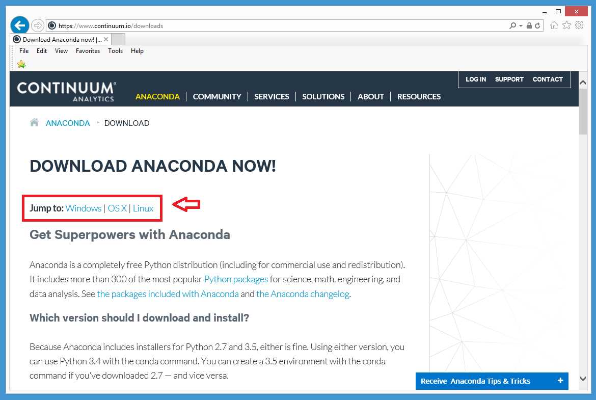
Figure 1: The Anaconda Download Site

Next, locate the link to your appropriate operating system and click on it.

At this point you must choose between Python version 2.x and Python version 3.x. If you're new to Python, the essential point is that the two versions are not fully compatible. Python users can have strong opinions about which Python version they prefer, but for use with SciPy, I recommend using Python 2.7 in order to maintain compatibility with older functions.

Figure 2: Python Version Selection

After selecting the Python version, you should see a message asking if you want to save the self-extracting executable installer, or if you want to run the installer immediately. You can do either. I chose the Run option.

Figure 3: Run the Executable Installer

The installation process begins by displaying a welcome splash screen. Notice that the Anaconda distribution number (2.4.1 in this case) is not the same as the Python version number (2.7).

Figure 4: The Welcome Splash

After clicking Next, you'll be presented with a license agreement, which you can read if you're a glutton for legal jargon punishment. Click I Agree.

Figure 5: License Agreement

Next, you'll have the option of installing for all users or just for the current user (presumably you). I suggest using Anaconda's recommendation.

Figure 6: User Options

Then, you'll need to specify the installation root directory. With open source software such as Python, it's normal to install programs in a directory located off drive C rather than in the C:\Program Files directory. I recommend installing at C:\Anaconda2.

Figure 7: The Installation Directory

Next, you'll get an option to add the locations of the Anaconda executables to the System PATH variable, and an option to register the Anaconda Python as the default. Select both check boxes and click Install.

Figure 8: The PATH and Integration Options

You'll see a progress bar during the installation process. Notice that NumPy and SciPy are included in the installation components.

Figure 9: Anaconda Includes SciPy and NumPy

When the installation is complete, you'll see an "Installation Complete" message. If there are any errors during the installation, they'll appear here. If so, you can read the error messages, fix whatever is wrong, delete the root installation directory, and try again.

Figure 10: Installation Completed

After you click Next, you'll see a final completion confirmation message. You can click Finish.

Figure 11: Installation Confirmation

The last step of the Anaconda installation process is to verify that your installation is working. First, verify that Python is up and running. Launch a command shell and navigate to the root directory by entering a cd \ command. Then type the command:

C:\> python --version

If Python responds with information about a version, then Python is almost certainly installed correctly, but you should now verify this by executing a Python statement. At the command prompt, enter the command python (I've included a space after the prompt for readability):

C:\> python

This will start the Python interpreter, which will be indicated by the three greater-than characters prompt. Instruct Python to print a traditional first message:

>>> print "Hello, Python!"

Finally, verify that NumPy is installed correctly by creating and manipulating an array. Enter the following commands at the Python prompt:

>>> import numpy as np
>>> a = np.array([4, 6, 8])
>>> print type(a)
>>> a[0] = 7
>>> print a
>>> exit()

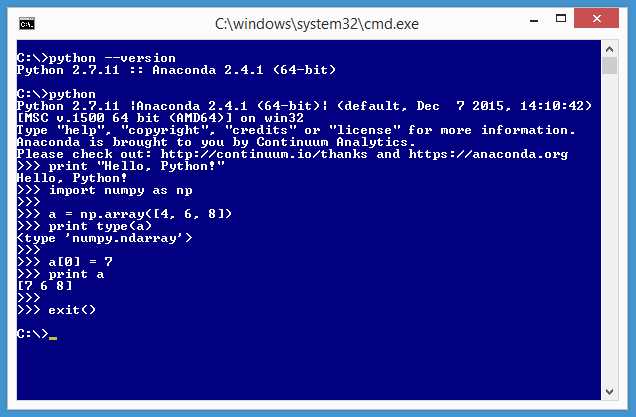
Figure 12: Verify Your Installation

The import statement brings the NumPy library into scope so it can be used. The np alias could have been something else, but np is customary and good.

The statement a = np.array([4, 6, 8]) creates an array named a with three cells with integer values 4, 6, and 8. The Python type() function tells you that a is, in fact, an array (technically an ndarray, which stands for an n-dimensional array).

The statement a[0] = 7 sets the value in the first cell of the array to 7, overwriting the original value of 2. The point here is that NumPy arrays, like those in most languages, use 0-based indexing. Congratulations! You have all the software you need to explore SciPy and NumPy.

Installing Python, NumPy, and SciPy Separately

Instead of using the Anaconda distribution, you can install Python, NumPy, and SciPy separately. To install Python, go to https://www.python.org/downloads/ and select the download for either a 3.x or 2.x version. I recommend the 2.7 version. After installation is complete, add C:\Python27 (or the location of python.exe if you used a non-default location) and C:\Python27\Lib\idelib to your system PATH environment variable. To install NumPy and SciPy, I strongly recommend that you use pre-built executable installers. In particular, the ones I recommend are maintained at the SourceForge repository. Install NumPy first. Go to http://sourceforge.net/projects/numpy/files/NumPy/.

That site has different versions of both NumPy and SciPy. Go into the directory of the version you wish to install. I recommend using a recent version that has the most downloads. Go into a version directory, and then look for a file named something like numpy-1.10.2-win32-superpack-python2.7.exe.

Figure 13: Binary Installer Link for NumPy

Make sure you have the version that corresponds to your Python version, then click on the link and you'll get the option to run the installer.

You'll have the option to either run the installer program immediately, or save the installer so you can run it later. I usually choose the Run option.

Figure 14: Run the NumPy Installer Executable

After you click Run, the installer will launch and present you with an installation wizard. Click Next.

Figure 15: NumPy Installation Wizard

The installer should find your existing Python installation and recommend an installation directory for the NumPy library.

Figure 16: The NumPy Installer Finds Existing Python Installation

Click Next on the next few wizard pages and you'll complete the NumPy installation. You can verify NumPy was installed by launching a Python shell and entering the command import numpy. If no error message results, NumPy has been installed.

Figure 17: Verify Separate NumPy Installation

Now you can install the SciPy library from SourceForge using the exact same process.

Resources

For installation information, including alternatives to the Anaconda distribution, see
http://www.scipy.org/install.html.

1.2 Editing SciPy Programs

Although Python and SciPy can be used interactively, for many scenarios you'll want to write and execute a program (technically a script). If you have installed the Anaconda distribution, you have three main ways to edit and execute a Python program. First, you can use any simple text editor, such as Notepad, and execute from a command line. Second, you can edit and execute programs using the IDLE (Integrated DeveLopment Environment) program. Third, you can edit and execute using the Spyder program. I'll walk you through each approach.

Code Listing 1: A Simple SciPy/NumPy Program

Launch Notepad and type or copy and paste the statements shown in Code Listing 1. Save the program as test.py in any directory, such as C:\SciPy. If you use Notepad, be sure it doesn't add an extra .txt extension to the file name.

Figure 18: Executing from a Command Prompt

Launch a Command Prompt (Windows) or command shell such as bash (Linux). Navigate to the directory containing file test.py. Execute the program by entering the command:

> python test.py

Using Notepad as an editor and executing from a shell is simple and effective, but I recommend using either IDLE or Spyder. The idle.bat launcher file is typically located by default in the C:\Python27\Lib\idelib directory. To start the IDLE program, launch a command shell, navigate to the location of the .bat file if that directory is not in your PATH variable, and enter the command idle.

This will start a special Python Shell as shown in the top part of Figure 19.

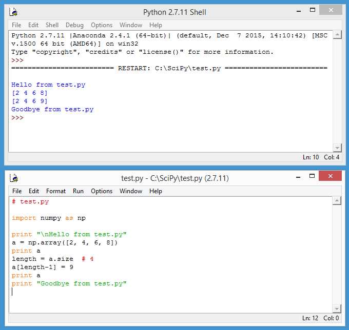
Figure 19: Using the IDLE Program

From the Python Shell menu bar, click File > New File. This will launch a similar-looking editor, as shown in the bottom part of Figure 19. Now, type or copy and paste the program in Code Listing 1 into the IDLE editor. Save the program as test.py in any convenient directory using File > Save. Execute the program by clicking Run > Run Module, or pressing the F5 shortcut key.

Program output is displayed in the Python Shell window. Some experienced Python users criticize IDLE for being too simple and lacking sophisticated editing and debugging features, but I like IDLE a lot and it's my SciPy programming environment of choice in most situations.

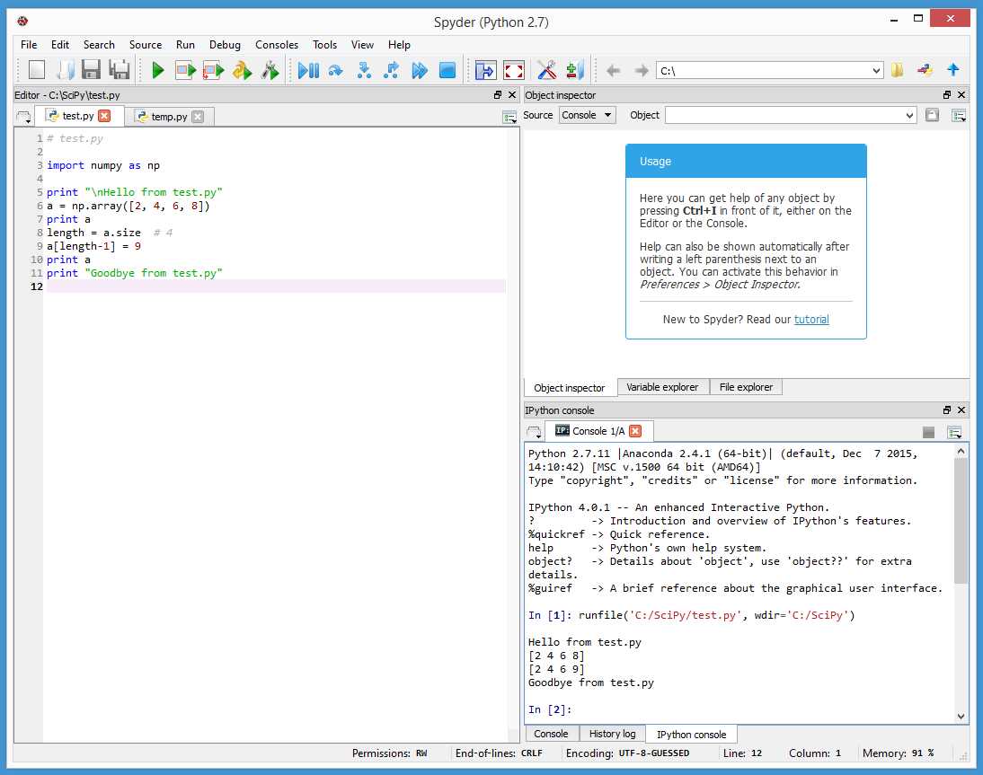
Figure 20: Using the Spyder Program

The Anaconda distribution comes with the open source Spyder (Scientific PYthon Development EnviRonment) program. To start Spyder, launch a command shell and enter:

> spyder

Type or copy and paste the program from Code Listing 1 into the Spyder editor window on the left side. You can either save first using File > Save or execute immediately by clicking Run > Run. Program output appears in the lower right window.

Resources

If you use Visual Studio, consider the Python Tools for Visual Studio (PTVS) plugin at
http://microsoft.github.io/PTVS/.

If you use the Eclipse IDE, you might want to take a look at the PyDev plugin at
http://www.pydev.org/.

1.3 Program Structure

Because the Python language is so flexible, there are many ways to structure a program. Some experienced Python programmers have strong opinions about what constitutes good Python program structure. Other programmers, like me, believe that there's no single best program structure suitable for all situations.

Take a look at the demo program in Code Listing 2. The program begins with comments indicating the program file name and Python version. Because the Python 2.x and Python 3.x versions are not fully compatible, it's a good idea to indicate which version your program is using. If you are using Linux, you can optionally use a shebang like #!/usr/bin/env python as the very first statement.

Code Listing 2: Python Program Structure Demo

Next, the demo program imports the NumPy library and assigns a short alias:

import numpy as np

This idiom is standard for NumPy and SciPy programming and I recommend that you use it unless you have a specific reason for not doing so. Next, the demo creates a program-defined function named make_x():

def make_x(n):
  result = np.zeros((n,n))
  for i in xrange(n):
    for j in xrange(n):
      if i == j or (i + j == n-1):
        result[i,j] = 1.0
  return result 

The make_x() function accepts a matrix dimension parameter n (presumably an odd integer) and returns a NumPy matrix with 1.0 values on the main diagonal (upper-left cell to lower-right cell) and the minor diagonal, and 0.0 values elsewhere.

The demo uses an indentation of two spaces instead of the widely recommended four spaces. I use two-space indentation throughout this e-book mostly to save space, but to be honest, I prefer using two spaces, anyway.

The demo program defines a main() function that is the execution entry point:

def main():
  print "\nBegin program structure demo \n"
  # rest of calling statements here
  print "\nEnd demo \n"

if __name__ == "__main__":
  main()

The program-defined main() function is called using the __main__ mechanism (note: there are two underscore characters before and after the word main). Defining a main() function has several advantages compared to simply placing the program's calling statements after import statements and function definitions.

The primary downside to using a main() function in your program is simply the extra time and space it takes you to write the program. Throughout the rest of this e-book, I do not use a main() function, just to save space.

By default, when the Python interpreter reads a source .py file, it will execute all statements in the file. However, just before beginning execution, the interpreter sets a system __name__ variable to the value __main__ for the source file that started execution. The value of the __name__ variable for any other module that is called is set to the name of the module.

In other words, the interpreter knows which program or module is the main one that started execution and will execute just the statements in that program or module. Put another way, Python modules that don't have an if __name__ == "__main__" statement will not be automatically executed. This mechanism allows you to write Python code and then import that code into another module. In effect, this allows you to write library modules.

Additionally, by using a main() function, you can avoid program-defined variable and function names clashing with Python system names and keywords. Finally, using a main() function gives you more control over control flow if you use the try-except error handling mechanism.

The demo program uses double quote characters to delimit strings. Unlike some other languages, Python recognizes no semantic difference between single quotes and double quotes. In particular, Python does not have a character data type, so both "c" and 'c' represent a string with a single character.

The demo program uses the try-except mechanism (that is, a try statement followed by an except statement). Using try-except is particularly useful when you are writing new code, but the downside is additional time and lines of code. The demo programs in the remainder of this e-book do not use try-except in order to save space.

Resources

The more or less official Python style guide is PEP 0008 (Python Enhancements Proposal #8). See https://www.python.org/dev/peps/pep-0008/.

Many Python programmers use the Google Python Style Guide. See
https://google.github.io/styleguide/pyguide.html.

For additional details about the Python try and except statements and error handling, see
https://docs.python.org/2/tutorial/errors.html.

For a discussion of the pros and cons of using a shebang in Linux environments, see
https://en.wikipedia.org/wiki/Shebang_(Unix).

1.4 Quick Reference Program

The program in Code Listing 3 is a quick reference for many of the NumPy and SciPy functions and programming techniques that are presented in this e-book.

Code Listing 3: Syntax Demo