Getting Started

The R programing language is designed to perform statistical analyses. Surveys of programming languages show that the use of R is increasing rapidly, apparently in conjunction with the increasing collection of data.

R can be used in two distinct ways. Most commonly, R is used as an interactive tool. For example, in an R console shell, a user could type commands such as:

> my_df <- read.table(“C:\\Data\\AgeIncome.txt”, header=TRUE)
> m <- lm(Income ~ Age, data=my_df)
> summary(m)

These commands would perform a linear regression data analysis of the age and income data stored in file AgeIncome.txt and would display the results of the analysis. R has hundreds of built-in functions that can perform thousands of statistical tasks.

However, you can also write R programs (i.e. scripts) by placing R commands and R language-control structures such as for-loops into a text file, saving the file, and executing the file. For example, a user can type commands such as:

> setwd(“C:\\Data\\MyScripts”)
> source(“neuralnet.R”)

These commands will run an R program named neuralnet.R, which is located in a C:\Data\MyScripts directory. You gain tremendous power and flexibility with the ability to extend the base R interactive functionality by writing R programs.

In this e-book, I will explain how to write R programs. I make no assumptions about your background and experience—even if you have no programming experience at all, you should be able to follow along with a bit of effort.

I will present a complete demo program in each section. Programmers learn how to program in a new language by getting an example program up and running, then experimenting by making changes. So, if you want to learn R programming, copy-paste the source code from a demo program, run the program, then make modifications to the program.

I will not present hundreds of one-line R examples. Instead, I will present short (but complete) programs that illustrate key R syntax examples and techniques. The code for all the demo programs can be found at https://github.com/jdmccaffrey/r-programming-succinctly.

In my experience, the most difficult part of learning any programming language or technology is getting a first program to run. After that, it’s just details. But getting started can be frustrating, and the purpose of this first chapter is to make sure you can install R and run a program.

Enough chit-chat already. Let’s get started.

1.1 Installing R

It’s no secret that the best way to learn a programming language or technology is to use it. Although you can probably learn quite a bit about R simply by reading this e-book, you’ll learn a lot more if you install R and run the demo programs that accompany each section.

Installing R is relatively quick and easy, and I’ll walk you through each step of the installation process for a Windows system. If you’re using a Linux system, the installation process varies quite a bit depending on which flavor of Linux you’re running, but there are many step-by-step installation guides available on the Internet. With Mac systems, R installation is very similar to Windows installation.

Launch a browser, search the Internet for “Install R,” and you’ll find a link for the Windows installer. At the time of this writing, the Windows installation URL is https://cran.r-project.org/bin/windows/base. Clicking the link will direct your browser to a page that resembles Figure 1.

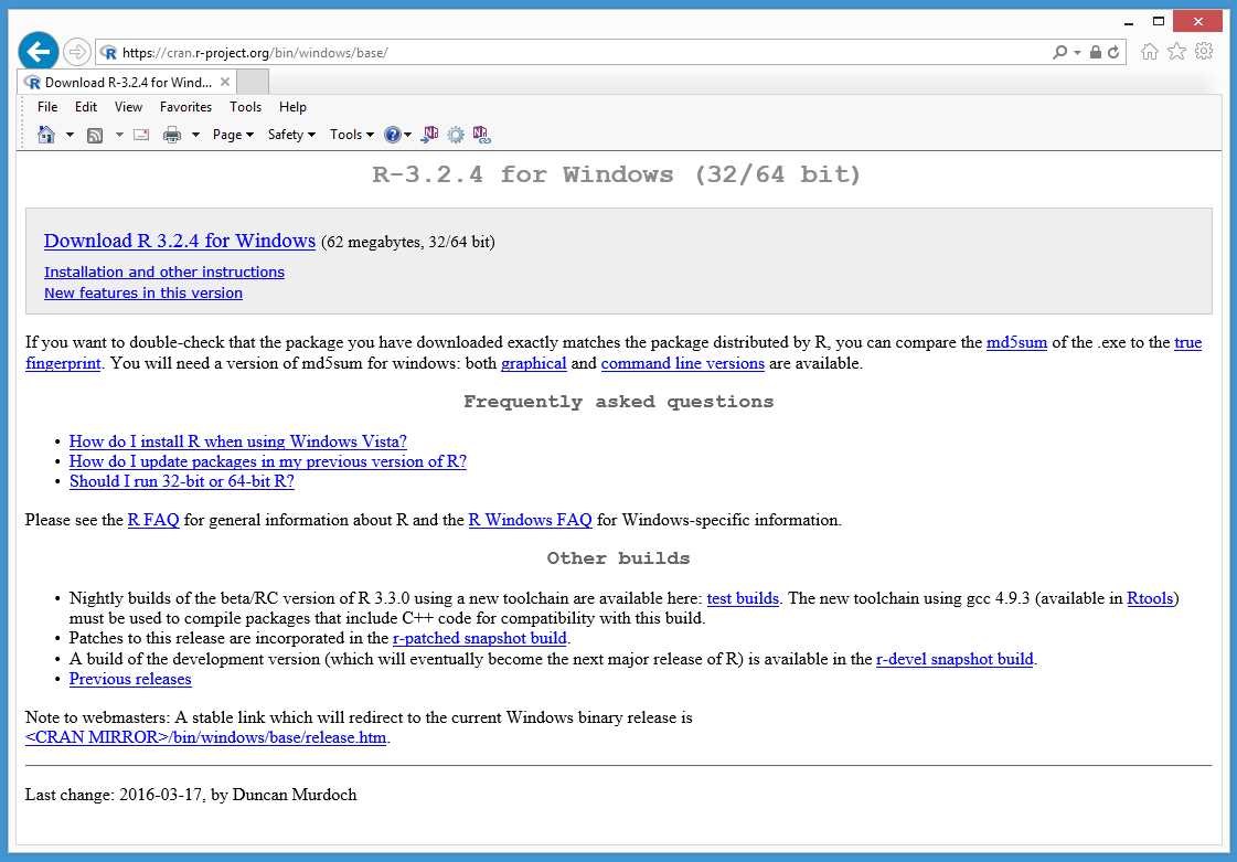
Figure 1: Windows Installation Page

The screenshot shows that I intend to install R version 3.2.4. By the time you read this, the most recent version of R will likely be different—however, the base R language is quite stable, and the code examples in this e-book have been designed to work with newer versions of R.

Notice the webpage title reads “(32/64 bit).” By default, on a 64-bit system (which you’re almost certainly using), the R installer will give you a 32-bit version of R and also a 64-bit version. The 32-bit version is for old machines and for backward compatibility with older R add-on packages that can only use the 32-bit version of R.

Next, click the link that reads “Download R 3.x.y for Windows.” The link points to a self-extracting executable installation program. Your browser will ask if you want to download the installer to your machine so that you can run the installation later, or it will ask if you want to run the install program immediately. Click “Run” to launch the installer.

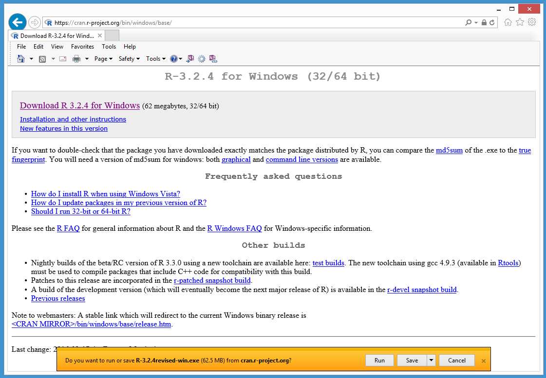
Figure 2: Run the Installer Now or Later

The installation program will start up and display a small dialog box asking you to select a language. One of R’s strengths is that it supports many different spoken languages. Select your language from the drop-down list and click “OK.”

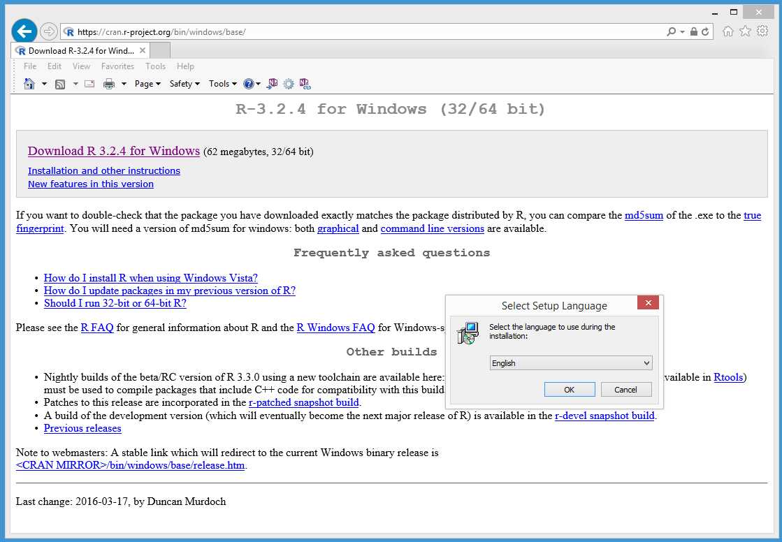
Figure 3: Select Language

Next, the installation program will display a Welcome window. Note that you will need administrative privileges on your machine in order to install R. Click “Next.”

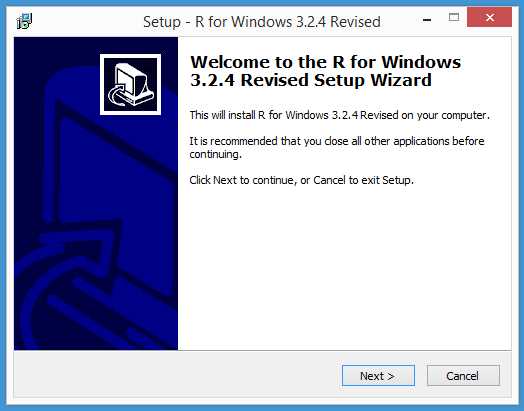
Figure 4: Installation Welcome Window

The installer will display the licensing information. If you look at the window scroll bar, you’ll notice there’s a lot of information. R runs under several different open source licenses. Read all the information if you’re a glutton for legal punishment or just click “Next.”

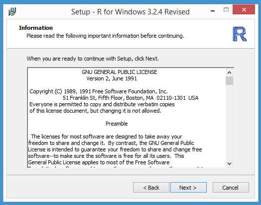
Figure 5: Licensing Information

Next, the installer will ask you to specify the installation directory. The default location is C:\Program Files\R\R-3.x.y, and I recommend you use the default location unless you have a good reason not to. Click “Next.”

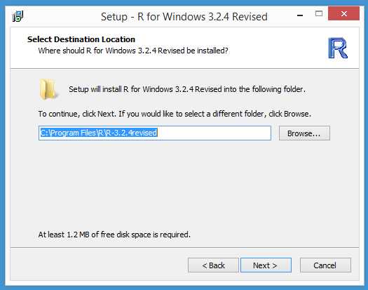
Figure 6: Specify the Installation Location

Next, the installer will ask you to select from four components. By default, all components are selected. Unless your machine has a memory shortage, you can leave all components selected and click “Next.” You need at least the core files and either the 32-bit files or the 64-bit files component.

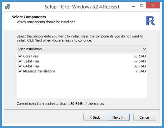
Figure 7: Select Components to Install

Next, the installer will give you the option to customize your startup options. These options are contained in a file named Rprofile.site, and they control items such as the default editor. I recommend accepting all the defaults and clicking “Next.”

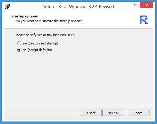
Figure 8: Specify the Startup Options

Next, the installer will ask where to place the program shortcuts. Accept the default location of “R” and click “Next.”

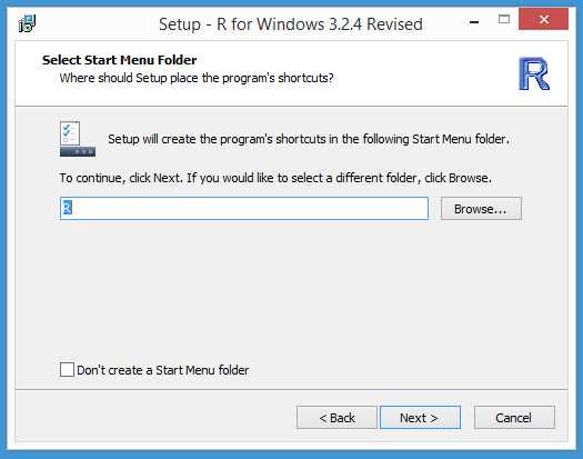
Figure 9: Select the Start Menu Folder

Next, the installer will ask you for some final options. The selected default options are fine—just click “Next.”

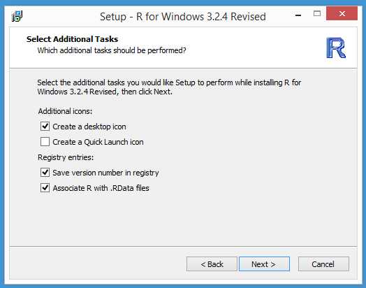
Figure 10: Additional Installation Options

Next, the actual installation process will begin. You’ll see a window that displays the installation progress. Installation is very quick—it should take no more than a minute or two.

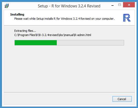
Figure 11: Installation Progress

When the install process completes, you’ll see a final window. Click “Finish” and you’ll be ready to start using R.

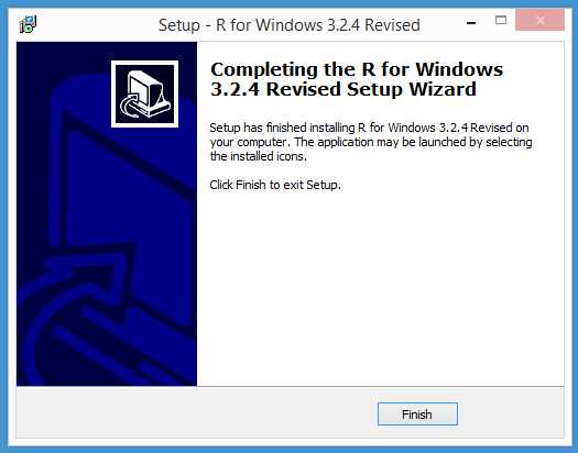
Figure 12: Installation is Complete

If you accepted the default install location, the R installation process places most of the key files at C:\Program Files\R\R-3.x.y\bin\x64. I recommend that you take a quick look there.

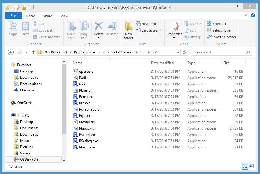
Figure 13: The Key R Files

In summary, installing R is relatively quick and easy. On a Windows system, the installer is a self-extracting executable. You can accept all the installation default options. The installation process will give you both a 32-bit version (primarily for backward compatibility with old add-on packages) and a 64-bit version.

1.2 Editing and running R programs

You can edit and execute an R program in several ways. If you are new to the R language, I recommend using the Rgui.exe program that is installed with R. Open a File Explorer window and navigate to the C:\Program Files\R\R-3.x.y\bin\x64 directory (or \i386 if you’re using an old 32-bit machine).

Locate the Rgui.exe file. You can double-click on Rgui.exe to launch it, or you can right-click the file, then select the “Run as administrator” option. For editing and running simple programs, you can simply double-click. However, if you need to install add-on packages, you must run Rgui.exe with administrative privileges.

After Rgui.exe launches, you’ll see an outer-shell window that contains an RConsole window. The RConsole window allows you to issue interactive commands directly to R. In order to create an R program, go to the menu bar and select File | New Script. This will create an R Editor window inside the shell window, where you can write an R program.

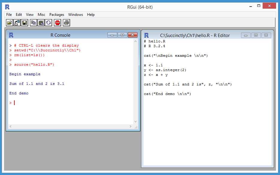
Figure 14: Using the Rgui.exe Program

In the R Editor window, type or copy-paste this code:

# hello.R
# R 3.2.4

cat(“\nBegin example \n\n”)

x <- 1.1
y <- as.integer(2)
z <- x + y

cat(“Sum of 1.1 and 2 is”, z, “\n\n”)
cat(“End demo \n\n”)

You must save the program before running it. Click File | Save As, then navigate to any convenient directory and save the program as hello.R. I saved my program at C:\Succinctly\Ch1.

To run the program, click anywhere on the RConsole window, which will give it focus. If you wish to erase all the somewhat annoying R startup messaging, you can do so by typing CTRL-L. Next, type the following commands in the RConsole window:

> setwd(“C:\\Succinctly\\Ch1”)
> rm(list=ls())
> source(“hello.R”)

The setwd() command sets the working directory to the location of the R program. Notice the required C-family language syntax of double backward slashes. Because R is multiplatform, you can also use single forward slashes if you wish.

The rm(list=ls()) command can be thought of as a magic R incantation that deletes all R objects currently in memory. You should always issue this command before running an R program. Failure to do so can lead to errors that are very difficult to track down.

The source() command is used to execute an R program. Technically, R programs are scripts because R is interpreted rather than compiled. However, I use the terms “program” and “script” interchangeably in this e-book.

After you make a change to your code, you can save using the standard shortcut CTRL-S or by selecting the File | Save option. When you close the Rgui.exe program, you’ll be presented with a dialog box that asks if you want to “Save workspace image?” You can click “No.”

A workspace image consists of the R objects currently in memory. Because a program recreates objects, saving the image isn’t necessary. Typically, you save an image when you’ve been using R interactively and have typed dozens or even hundreds of commands, and you don’t want to lose the state of all the objects you’ve created. If you do save an R image, the image is saved with a .RData file extension. Workspace images can be restored by using the File | Load Workspace menu option.

In summary, I recommend using the Rgui.exe program in order to write and execute an R program. You write and edit programs in an Editor window and run programs by issuing a source() command in the RConsole window. There are dozens of alternatives for editing R programs. I sometimes use the open source Notepad++ program to write R programs because it gives me nice source code coloring. Some of my colleagues use the open source RStudio program.

Resources

The source() function has many useful options to control running an R program. See:
https://stat.ethz.ch/R-manual/R-devel/library/base/html/source.html.

1.3 Using add-on packages

The R language is organized into packages. When you install R, you get about 30 packages with names like base, graphics, and stats. These built-in packages allow you to perform many programming tasks, but you can also install and use hundreds of packages that have been created by the R community.

Add-on packages are both a strength and weakness of R. Because anyone can write an R package, quality can vary greatly. And because packages can have dependencies on other packages, if you install lots of packages, it’s possible that you’ll run into versioning problems. In order to avoid this, in this e-book I use only the built-in R packages that come with the R install.

You can issue the command installed.packages() in the R Console window in order to see which packages are currently installed on your system. Note that unlike most programming languages, R often uses the “.” character rather than the “_” character as part of a function name, which makes the name more readable. If you are an experienced programmer, this syntax can be surprisingly difficult at first.

In order to install a package, you use the install.packages() function. For example, there is the BigInteger data type. When installing the gmp add-on package, make sure you’re connected to the Internet, then type the command install.packages(“gmp”). This will launch a small window that allows you to select a website from which to install the gmp package.

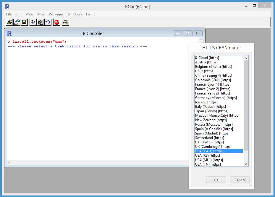
Figure 15: Selecting a Mirror when Installing an Add-On Package

You can select any of the mirror websites, then click “OK.” The package installation process is silent and generally relatively quick. On rare occasions, the installation process will fail, typically because the mirror website is down or the mirror site doesn’t have the requested package. If this happens, you’ll get an error message. You can try a different mirror site by issuing the command chooseCRANmirror().

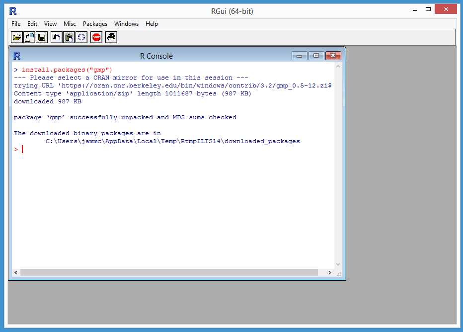
Figure 16: Package Installed Successfully

After your add-on package has been installed successfully, you access the package by using the library() or require() function. For example, in an interactive mode, you can type the command library(gmp), then you can use all the functions and classes defined in the gmp package. For example, these commands will display the value of 20 factorial (as shown in Figure 17):

> library(gmp)
> f = factorialZ(20)
> f

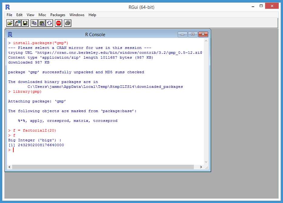
Figure 17: Accessing an Add-On Package

Both the library() function and the require() function load an installed package into the current context, but library() will return an error and halt execution if the target package is not installed. However, require() will return a value of FALSE and attempt to continue execution if the target package is not installed. After you finish using an add-on package, you should consider uninstalling the package in order to prevent your system from becoming overwhelmed with packages.

In order to remove a package, first list the installed packages using the installed.packages() function. In most cases, when removing packages, you’ll want to list all installed packages because you might have several instances of the same package that contain different versions. You can list just a few of the installed packages or just some of the information about each by specifying the number of rows and columns in the output. For example, the command installed.packages()[1:5,1:3] will list rows 1-5 of the installed packages table with columns 1-3 of the table information. In order to remove a package, use the remove.packages() function; for example, remove.packages(“gmp”) or remove.packages(“gmp”, version=“0.5-12”).

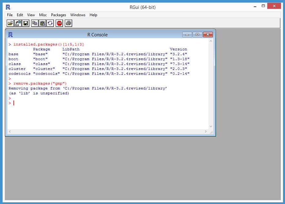
Figure 18: Removing a Package

In summary, installing R gives you about 30 built-in packages that contain most of the functionality you need for common programming tasks. In order to manage add-on packages, you can use the installed.packages(), install.packages(), and remove.packages() functions. In order to access an add-on package, you can use either the library() function, which will fail if the requested package is not installed on your system, or the require() function.

Resources

For details about the differences between the library() and require() functions, see:
https://stat.ethz.ch/R-manual/R-devel/library/base/html/library.html.

1.4 R Syntax and style reference program

The program in Code Listing 1 gives a quick reference for the syntax of common R language features such as if-then and for-loop statements.

Code Listing 1: R Language Syntax Examples

If you’re new to R, a few syntax quirks might be confusing. In R, there are two assignment operators: the <- operator and the = operator. In most situations, either assignment operator can be used.

The R language is one of the few languages in which vectors, arrays, and lists use 1-based indexing rather than 0-based indexing.

In an if-then-else statement, curly braces are required even in the case of a single then-statement. Inside a function definition, you can use the easier-to-read C-style in which the else keyword and the right curly brace from the if appear on separate lines. However, outside of a function definition, you must use R-style when the else and the right curly brace are on the same lines.

Although several R language style guidelines have been proposed and published, there is little agreement in the R community about what constitutes good R language style. In my opinion, consistency and common sense are more important than a slavish attention to any style guide. 

In summary, R language syntax is quite similar to the C language. R uses both the <- and = operators for assignments (there’s also a specialized <<- operator used with reference classes). R collections are 1-based rather than 0-based. You can use easy-to-read, if-then C-style syntax inside a function definition, but you must use R-style syntax outside a code block definition.

Resources                                                                             

The official R language definition can be found at:
https://cran.r-project.org/doc/manuals/r-release/R-lang.html.