Advanced R Programming

---

The R programming language contains all the features needed to create very sophisticated programs. This chapter presents three topics (random number generation, neural networks, and combinatorial optimization) that illustrate the power of R, demonstrate useful R programming techniques, and give you starting points for a personal code library. Figure 22 gives you an idea of where this chapter is headed.

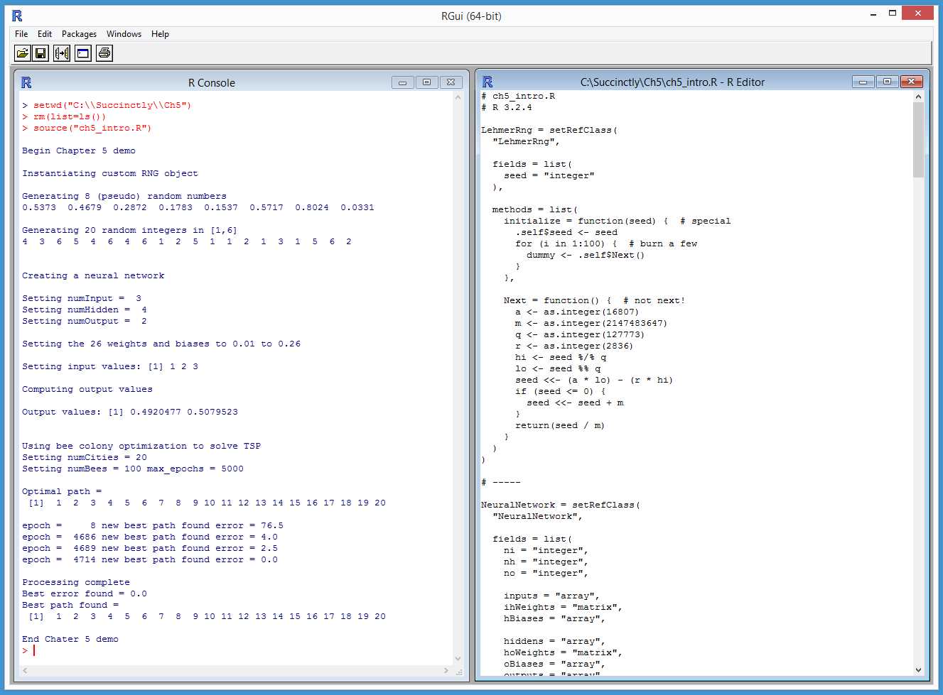
Figure 22: Advanced R Programming Topics

In section 5.1, you’ll learn how to create a program-defined random number generator (RNG) object using an RC model and the Lehmer random number generation algorithm.

In section 5.2, we’ll look at how to design and create a neural network and how to write code that implements the neural network feed-forward, input-process-output mechanism.

In section 5.3, you’ll learn how to solve combinatorial optimization problems using a bio-inspired algorithm that models the behavior of honey bees. In particular, you’ll come to understand how to solve the traveling salesman problem, arguably the most well-known combinatorial-optimization problem.

5.1 Program-defined RNGs

Most programming languages allow you to create multiple instances of random number generators. The R language uses a single, global-system RNG that is somewhat limiting. However, you can write your own RNG class in R.

Code Listing 15: A Random Number Generator Class

Here is an example of creating RNGs with other programming languages:

Random my_rng = new Random(0);  // C# and Java
my_rnd = random.Random(0)  # Python

There are many different RNG algorithms. Among the most common are the linear congruential algorithm, the Lehmer algorithm, the Wichmann-Hill algorithm, and the Lagged Fibonacci algorithm. The demo program uses the Lehmer algorithm and creates a Reference Class definition named LehmerRng. Here is the structure of the class:

LehmerRng = setRefClass(
  “LehmerRng”,
  fields = list( . . . ),
  methods = list( . . . )
)

The Lehmer algorithm is X(i+1) = a * X(i) mod m. In English, that is “the next random value is some number a times the current value modulo some number m.” For example, suppose the current random value is 104, where a = 3 and m = 100. The next random value would be 3 * 104 mod 100 = 312 mod 100 = 12. It’s standard practice for RNGs to return a floating-point value between 0.0 and 1.0, so the next-function of the RNG would return 12 / 100 = 0.12.

The next random value would be 3 * 12 mod 100 = 36, and the next-function would emit 0.36. The X(i) in most RNG algorithms is named “seed.” The fields part of the LehmerRng class definition is simply:

fields = list(
  seed = “integer”
),

The custom RNG contains two methods. The Next() function implements the Lehmer algorithm but uses an algebra trick to prevent arithmetic overflow:

Next = function() {
  a <- as.integer(16807)
  m <- as.integer(2147483647)
  q <- as.integer(127773); r <- as.integer(2836)
  hi <- seed %/% q; lo <- seed %% q
  seed <<- (a * lo) - (r * hi)
  if (seed <= 0) { seed <<- seed + m }
  return(seed / m)
}

Integer values a and m are the multiplier and modulo constants. Their values come from math theory, and you should not change them. The q value is (m / a) and the r value is (m mod a). By using q and r, the algorithm prevents arithmetic overflow during the a * X(i) multiplication part of the algorithm. Local variables a, m, q, and r could have been defined as class fields.

I use Next() upper case rather than next() lower case because next is a reserved word in R (used to short-circuit to the next iteration of a for-loop). The class definition also has the special Reference Class initialize() function:

initialize = function(seed) {
  .self$seed <- seed
  for (i in 1:100) {  # burn a few
    dummy <- .self$Next()
  }
},

If you define an initialize() function in an S4 or RC class, control will be transferred to initialize()  when you instantiate an object of the class using the new() function. Here, the initialize() function sets the seed field, then generates and discards the first 100 values. Notice the use of the .self keyword to access the seed field and the Next() function.

The seed value could have been set with:

seed <<- seed

Here, the seed on the left side of the <<- assignment operator is the class field, and the seed on the right side of the assignment is the input parameter. But that syntax looks a bit odd. Whenever I set a field value using a parameter with the same name, I like to use the explicit .self syntax. Notice, however, that when you do assign an RC class field value using .self, you must use the regular <- assignment operator rather than the <<- assignment operator.

The demo program instantiates an object this way:

my_rng <- LehmerRng$new(as.integer(1))

An initial seed value of 1 is passed to the new() function. Some RNG algorithms can use an initial seed value of 0, but the initial seed must be 1 or greater for the Lehmer algorithm, which means you could add an error-check to the initialize() function. Because the class has a defined initialize() function, control is passed from new() to initialize(). The input parameter value of 1 is assigned to the seed field, and then the first 100 random values are generated and discarded. Burning a few hundred or a few thousand initial values is a common technique in RNG implementations.

The demo program uses the RNG object to generate a few random floating-point values:

for (i in 1:8) {
  x <- my_rng$Next()
  xx <- formatC(x, digits=4, format=“f”)
  cat(xx, “ “)
}

The demo program shows how to map random floating-point values between 0.0 and 1.0 to integers between [1, 6] inclusive this way:

lo <- as.integer(1)
hi <- as.integer(7)  # note: 1 more than 6
for (i in 1:20) {
  n <- floor((hi - lo) * my_rng$Next() + lo)
  cat(n, “ “)
}

In summary, if you want multiple, independent random-number generator objects, you can define your own RC class. If you define the optional initialize() function, when assigning a field value that has the same name as an input parameter, consider using the .self syntax.

Resources

An excellent, famous paper that describes how to implement the Lehmer RNG algorithm is:
http://www.firstpr.com.au/dsp/rand31/p1192-park.pdf.

For additional information about the Lehmer RNG algorithm, see:
https://en.wikipedia.org/wiki/Lehmer_random_number_generator.

5.2 Neural networks

This section explains the input-process-output mechanism of an R language implementation of a neural network. This mechanism is called neural network feed-forward.

Code Listing 16: A Neural Network

Let’s think of a neural network as a complicated math function that accepts numeric input values, does some processing in a way that loosely models biological neurons, and produces numeric output values that can be interpreted as predictions.

Here are the key lines of demo program code that create a neural network:

numInput <- as.integer(3)
numHidden <- as.integer(4)
numOutput <- as.integer(2)

nn <- NeuralNetwork$new(numInput, numHidden, numOutput)

The number of input and output nodes is determined by the prediction problem. The number of hidden nodes is a free parameter and must be determined by trial and error.

The demo neural network has three input nodes, four hidden nodes, and two output nodes. For example, if you’re trying to predict whether a person is a political conservative or liberal (two output possibilities) based on income level, education level, and age level (three input values).

After the neural network object is created, it is initialized with these lines of code:

wts <- seq(0.01, 0.26, by=0.01)
nn$setWeights(wts)

A neural network has constants called weights and biases that, along with the input values, determine the output values. A neural network that has x input nodes, y hidden nodes, and z output nodes has (x * y) + y + (y * z) + z weights and biases. That means the demo 3-4-2 network has (3 * 4) + 4 + (4 * 2) + 2 = 26 weights and biases. The demo generates 26 values from 0.01 to 0.26 using the built-in seq() function, then uses a class function/method setWeights() to copy the values into the neural network’s weights and biases.

The demo computes output values for an input set of (1.0, 2.0, 3.0) with this code:

xValues <- c(1.0, 2.0, 3.0)
outputs <- nn$computeOutputs(xValues)
print(outputs)

The two output values are (0.4920, 0.5080). This diagram shows the conceptual structure of the demo neural network:

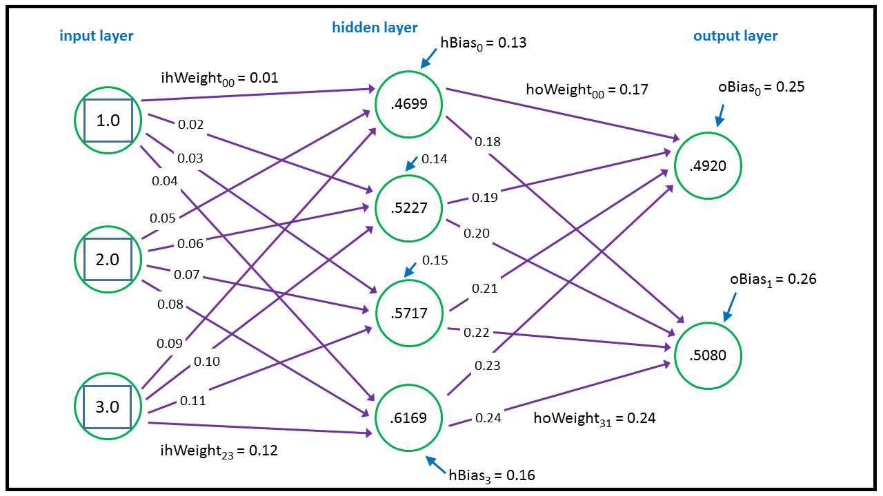
Figure 23: Neural Network Architecture

Each purple line connecting a pair of nodes represents a weight. Additionally, each of the hidden and output nodes (but not input nodes) has a blue arrow that represents a bias. The neural network calculates its outputs from left to right. The top-most hidden node value is calculated:

tanh( (1.0 * 0.01) + (2.0 * 0.05) + (3.0 * 0.09) + 0.13 ) = tanh(0.51) = 0.4699

The tanh (hyperbolic tangent) is called the activation function in neural network terminology. In words, we’d say “in order to calculate a hidden node value, you multiply each input value times the associated input-to-hidden weight, sum, add the hidden node bias value, and then take the tanh of the sum.”

The values of the two output nodes are calculated a bit differently. First, preliminary sums are calculated:

oSums[1] = (0.46 * 0.17) + (0.52 * 0.19) + (0.57 * 0.21) + (0.61 * 0.23) + 0.25 = 0.69
oSums[2] = (0.46 * 0.18) + (0.52 * 0.20) + (0.57 * 0.22) + (0.61 * 0.24) + 0.26 = 0.72

Then these values are used to determine the final output values by using a special function called the softmax function:

outputs[] = softmax(oSums[1], oSums[2]) = (0.4920, 0.5080)

These output values can be interpreted as probabilities. In this case, because the second value is (just barely) larger than the first value, the neural network predicts that a person with an income level of 1.0, an education level of 2.0, and an age level of 3.0 is a liberal (the second outcome possibility).

Here is the structure of the demo neural network RC class:

NeuralNetwork = setRefClass(
  “NeuralNetwork”,
  fields = list( . . . ),
  methods = list( . . .)
)

These are the class fields:

fields = list(
  ni = “integer”, nh = “integer”, no = “integer”,
  inputs = “array”,
  ihWeights = “matrix”,
  hBiases = “array”,

  hiddens = “array”,
  hoWeights = “matrix”,
  oBiases = “array”,
  outputs = “array”
),

Fields ni, nh, and no are the number of input, hidden, and output nodes. Matrix ihWeights holds the input-to-hidden weights where the row index corresponds to an input node index, and the column index corresponds to a hidden node index. Array hBiases holds the hidden node bias values. Matrix hoWeights holds the hidden-to-output weights, and array oBiases holds the output node biases.

The initialize() function is defined as:

initialize = function(ni, nh, no) {
  .self$ni <- ni
  .self$nh <- nh
  .self$no <- no

  inputs <<- array(0.0, ni)
  ihWeights <<- matrix(0.0, nrow=ni, ncol=nh)
  hBiases <<- array(0.0, nh)

  hiddens <<- array(0.0, nh)
  hoWeights <<- matrix(0.0, nrow=nh, ncol=no)
  oBiases <<- array(0.0, no)
  outputs <<- array(0.0, no)
},

Although all the fields defined as array types could be made vectors, it’s more principled to use the array type when interoperating with matrix objects.

If you modify a field in an RC class using the .self syntax, you use the <- assignment operator, but if you don’t qualify a field with .self, you must use the <<- assignment operator.

The definition of class method setWeights() begins as:

setWeights = function(wts) {
  numWts <- (ni * nh) + nh + (nh * no) + no
  if (length(wts) != numWts) {
    stop(“FATAL: incorrect number weights”)
  }
. . .

Function setWeights() accepts an array or vector of all the weights and biases. If the number of weights and biases in the input wts parameter isn’t correct, the function calls the built-in stop() function to halt program execution immediately. Function setWeights() continues by setting an index, wi, into the wts array/vector parameter, then populates the input-to-hidden weights matrix in row-order form (left to right, top to bottom):

wi <- as.integer(1)
for (i in 1:ni) {
  for (j in 1:nh) {
    ihWeights[i,j] <<- wts[wi]
    wi <- wi + 1
  }
}

Notice that the <<- assignment operator is needed to modify the member matrix, but ordinary <- assignment is used for the wi local variable. Function setWeights() finishes by copying value from the wts parameter into the hidden node biases, followed by the hidden-to-output weights, and finally to the output node biases:

for (j in 1:nh) {
  hBiases[j] <<- wts[wi]
  wi <- wi + 1
}

for (j in 1:nh) {
  for (k in 1:no) {
    hoWeights[j,k] <<- wts[wi]
    wi <- wi + 1
  }
}

for (k in 1:no) {
  oBiases[k] <<- wts[wi]
  wi <- wi + 1
}

In short, the setWeights() function deserializes its input array/vector values first to the input-to-hidden weights matrix in row-order fashion, then to the hidden node biases, then to the hidden-to-output weights matrix in row-order fashion, and finally to the output node biases. There is no standard order for copying weights, and if you’re working with another neural network implementation, you must check to see exactly which ordering is being used.

The definition of member function computeOutputs() begins with:

computeOutputs = function(xValues) {
  hSums <- array(0.0, nh) # hidden nodes scratch array
  oSums <- array(0.0, no) # output nodes scratch
  for (i in 1:ni) {
    inputs[i] <<- xValues[i]
  }
. . .

Local array hSums holds the pre-tanh activation sums for the hidden nodes. Local array oSums holds the pre-softmax activation sums for the output nodes. The values in the input parameter xValues array/vector are then copied into the neural network’s input array.

The values for the hidden nodes are computed with these lines of code:

for (j in 1:nh) {
  for (i in 1:ni) {
    hSums[j] <- hSums[j] + (inputs[i] * ihWeights[i,j])
  }
}
for (j in 1:nh) {
  hSums[j] <- hSums[j] + hBiases[j]
}
for (j in 1:nh) {
  hiddens[j] <<- tanh(hSums[j])
}

As explained earlier, first a sum of the products of input value times associated weight is computed, then the bias is added, then the tanh() activation function is applied.

The output values are calculated and returned this way:

for (k in 1:no) {
  for (j in 1:nh) {
    oSums[k] <- oSums[k] + (hiddens[j] * hoWeights[j,k])
  }
}
for (k in 1:no) {
  oSums[k] <- oSums[k] + oBiases[k]
}
outputs <<- my_softMax(oSums)
return(outputs)

Notice that unlike the hidden nodes, in which values are calculated one at a time, the output node values are calculated together by the my_softMax() program-defined function. The softmax function of one of a set of values is the exp() of that value divided by the sum of the exp() of all the values. For example, in the demo, the pre-softmax activation-output sums are (0.6911, 0.7229). The softmax of the two sums is:

output[1] = exp(0.6911) / (exp(0.6911) + exp(0.7229)) = 0.4920
output[2] = exp(0.7229) / (exp(0.6911) + exp(0.7229)) = 0.5080

The purpose of the softmax output-activation function is to coerce the output values so that they sum to 1.0, then can be loosely interpreted as probabilities, which in turn can be used to determine a prediction.

The feed-forward, input-process-output mechanism is just one part of a neural network. The next key part, which is outside the scope of this e-book, is called training the network. In the example neural network, the weights and biases values were set to 0.01 through 0.26 in order to demonstrate how feed-forward works. In a real neural network, you must determine the correct values of the weights and biases so that the network generates accurate predictions.

Training is accomplished by using a set of data that has known input values and known, correct output values. Training searches for the values of the weights and biases so that the computed outputs closely match the known, correct output values. There are several neural network training algorithms, but the most common is called the back-propagation algorithm.

In summary, it is entirely possible to implement a custom neural network, and an R Reference Class is well suited for an implementation. When writing an initialize() function, use the .self syntax for fields that have the same name as their associated parameters and use the <- assignment operator rather than the <<- operator.

Resources

For details about the relationship between the new() and initialize() functions, see:
https://stat.ethz.ch/R-manual/R-devel/library/methods/html/refClass.html.

5.3 Bee colony optimization

A combinatorial-optimization problem occurs when the goal is to arrange a set of items in the best way. The traveling salesman problem (TSP) is arguably the most well-known combinatorial-optimization problem, and bee colony optimization (BCO), an algorithm that loosely models the behavior of honey bees, is used to find a solution for TSP. 

Code Listing 17: Bee Colony Optimization

In using BCO to find a solution to TSP, the demo sets up a problem in which 20 cities exist and the goal is to find the shortest path that visits all 20 cities. The demo creates a problem by defining a make_data() function and an associated error() function. Code Listing 18 shows the function make_data() definition.

Code Listing 18: Programmatically Generating TSP City-to-City Distances

The function accepts a parameter nc—the number of cities. The return object is a matrix that defines the distance between two cities in which the row index is the “from” city and the column index is the “to” city. Every city is connected to every other city. The distance between two consecutive cities is best explained with examples: distance(3, 4) = 1.0; distance(4, 3) = 1.5; and distance(5, 5) = 0.0.

When defined this way, the optimal path that visits all 20 cities is 1 -> 2 -> . . -> 20. This path has a total distance of 19.0. In a realistic scenario, the distances between cities would probably be stored in a text file, and you’d write a helper function for reading the data from the file into a matrix.

Here is the associated error() function:

error = function(path, distances) {
  nc <- nrow(distances)
  mindist <- nc - 1
  actdist <- 0
  for (i in 1:(nc-1)) {
    d <- distances[path[i], path[i+1]]
    actdist <- actdist + d
  }
  return(actdist - mindist)
} 

The function accepts a path that has 20 city indices, walks through the path, and accumulates the total distance using the information in the distances matrix. The optimal-path distance is subtracted from the actual-path distance to give an error value.

In most realistic scenarios, you won’t know the optimal solution to your problem, which means you can’t define an error function as optimal minus actual. An alternative approach is to define error as a very large value (such as .Machine$integer.max) minus actual.

BCO is a metaheuristic rather than a prescriptive algorithm. This means BCO is a set of general design guidelines that can be implemented in many ways. The demo program models a collection of synthetic bees. Each bee has a path to a food source and an associated measure of that path’s quality. There are two kinds of bees—worker bees try different paths in a controlled fashion, and scout bees try random paths.

The demo program defines a Bee object using an S4 class:

Bee = setClass(
  “Bee”,
  slots = list(
    type = “integer”, #1 = worker, 2 = scout
    path = “vector”,
    error = “numeric”
  )
)

The Bee class has data fields but no class functions/methods. The Bee object types are hard-coded as 1 for a worker and 2 for a scout. In many programming languages you’d use a symbolic constant, but R does not support this feature.

All of the work is done by a program-defined solve() function. Expressed in high-level pseudocode, this is the algorithm used:

initialize a collection of bees with random path values
loop max_epochs times
  loop each bee
    if bee is a worker then
      examine an adjacent path
      if adjacent path is better, update bee
    else if bee is a scout then
      examine a random path
      pick a worker bee at random
      communicate the random path to the worker (“waggle”)
  end loop each bee
end loop max_epochs
display best path found

The definition of function solve() begins with:

solve = function(nc, nb, distances, max_epochs) {
  numWorker <- as.integer(nb * 0.80)
  numScout <- nb - numWorker
  hive <- list()
. . .

The total number of bees, nb, is passed in as a parameter. The number of worker bees is set to 80% of the total, and the rest are scout bees, although you can experiment with other percentages. The collection of Bee objects is stored in a list object. Even though the total number of bees is known, when working with collections of S4 or RC objects, I find it preferable to use a variable-length list object rather than a fixed-length vector object.

The Bee objects are initialized this way:

for (i in 1:nb) {
  b <- new(“Bee”)
  if (i <= numWorker) {
    b@type <- as.integer(1) # worker
  }
  else {
    b@type <- as.integer(2) # scout
  }

  b@path <- sample(1:nc)
  b@error <- error(b@path, distances)
  hive[[i]] <- b # place bee in hive
}

The built-in sample() function is used to generate a random permutation. The associated error of the random path is computed and stored. Notice the double-square bracket notation.

After all the Bee objects have been initialized, they are examined to find the best initial path and associated error:

best_error <- 1.0e40 # really big
best_path <- c(1:nc) # placeholder path
for (i in 1:nb) {
  if (hive[[i]]@error < best_error) {
    best_error <- hive[[i]]@error
    best_path <- hive[[i]]@path
  }
}

This initialize-best-path logic could have been placed inside the preceding initialization loop, but it’s a bit cleaner to use separate loops. The main while-loop processes each bee in the hive object. Here is the code in which a worker bee generates a neighbor path to the current path:

neigh_path <- hive[[i]]@path
ri <- sample(1:nc, 1)
ai <- ri + 1
if (ai > nc) { ai <- as.integer(1) }
tmp <- neigh_path[[ri]]
neigh_path[[ri]] <- neigh_path[[ai]]
neigh_path[[ai]] <- tmp
neigh_err <- error(neigh_path, distances)

Variable ri is a random index. Variable ai is an adjacent index that is only one greater than the random index. You might want to investigate an alternative design by defining a neighbor path as one in which the cities at two randomly selected indices are exchanged. Or you could define two different types of worker bees that have different neighbor-generation strategies.

Here is the code in which a Bee object’s path is updated:

p <- runif(1, min=0.0, max=1.0)
if (neigh_err < hive[[i]]@error || p < 0.05) {
  hive[[i]]@path <- neigh_path
  hive[[i]]@error <- neigh_err
. . .

A probability is generated and, 5% of the time, the path is updated even if the neighbor path is not better than the current path. This helps prevent bees from getting stuck at local minima.

In summary, BCO is a bio-inspired, swarm-intelligence metaheuristic that can be used to solve combinatorial problems. Swarm algorithms can use a list of S4 objects.   

Resources

For additional information about bee colony optimization, see:
https://en.wikipedia.org/wiki/Bees_algorithm.