Graphics Operators

In addition to text, PDFs are also a reliable format for the accurate reproduction of vector graphics. In fact, the Adobe Illustrator file format (.ai) is really just an extended form of the PDF file format. This chapter introduces the core components of the PDF graphics model.

The Basics                                               

Like text operators, graphics operators only provide the low-level functionality for representing graphics in a page’s content stream. PDFs do not have “circles” and “rectangles”—they have only paths.

Drawing paths is similar to drawing text, except instead of positioning the text cursor, you must construct the entire path before painting it. The general process for creating vector graphics is:

1. Define the graphics state (fill/stroke colors, opacity, etc.).
2. Construct a path.
3. Paint the path onto the page.

For example, the following stream draws a vertical line down the middle of the page:

First, this sets the stroke width to 10 points with the w operator. Then, we begin constructing a path by moving the graphics cursor to the point (306, 396) with m. This is similar to the Td command for setting the text position. Next, we draw a line from the current position to the point (306, 594) using the l (lowercase L) operator. At this point, the path isn’t visible—it’s still in the construction phase. The path needs to be painted using the S operator. All paths must be explicitly stroked or filled in this manner.

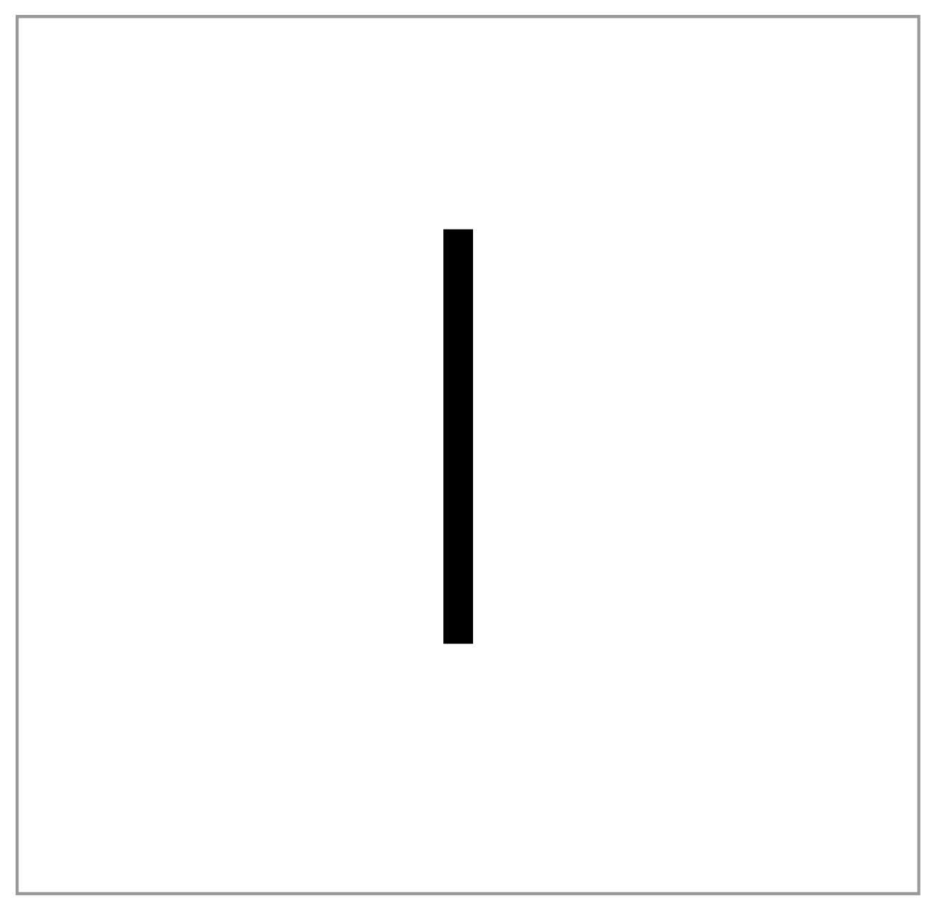
Figure 14: Screenshot of the previous stream (not drawn to scale)

Also notice that graphics don’t need to be wrapped in BT and ET commands like text operators.

Next, we’ll take a closer look at common operators for each phase of producing graphics.

Graphics State Operators

Graphics state operators are similar to text state operators in that they both affect the appearance of all painting operations. For example, setting the stroke width will determine the stroke width of all subsequent paths, just like Tf sets the font face and size of all subsequent text. This section covers the following graphics state operators:

• <width> w: Set the stroke width.
• <pattern> <phase> d: Set the stroke dash pattern.
• <cap> J: Set the line cap style (endpoints).
• <cap> j: Set the line join style (corners).
• <limit> M: Set the miter limit of corners.
• <a> <b> <c> <d> <e> <f> cm: Set the graphics transformation matrix.
• q and Q: Create an isolated graphics state block.

The w Operator

The w operator defines the stroke width of future paths, measured in points. Remember though, PDFs don’t draw the stroke of a path as it is being constructed—that requires a painting operator.

The d Operator

The d operator defines the dash pattern of strokes. It takes two parameters: an array and an offset. The array contains the dash pattern as a series of lengths. For example, the following stream creates a line with 20-point dashes with 10 points of space in between.

A few dash examples are included in the following figure. The last one shows you how to reset the dash state to a solid line.

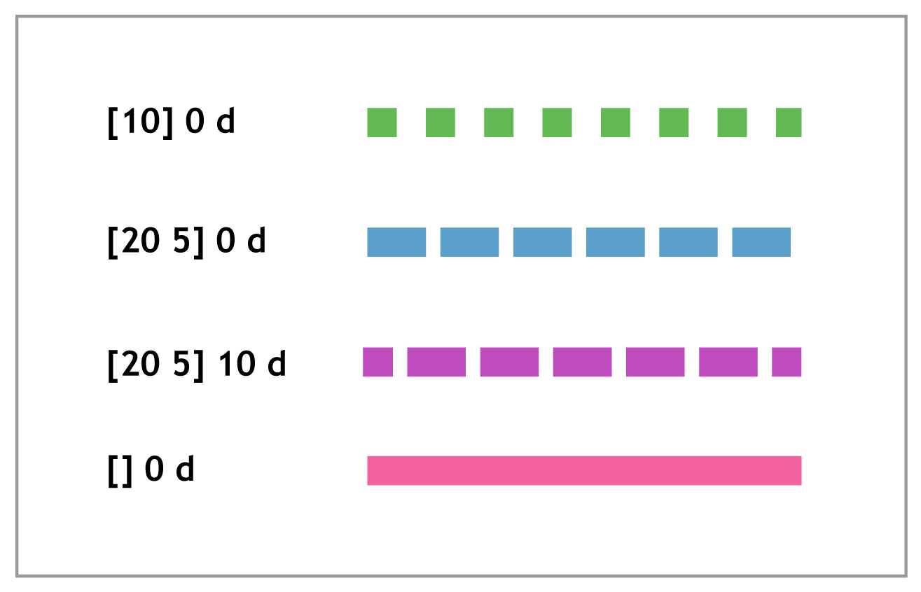
Figure 15: Dashed lines demonstrating the behavior of d

The J, j, and M Operators

All three of these operators relate to the styling of the ends of path segments. The J operator defines the cap style, and j determines the join style. Both of them take an integer representing the style to use. The available options are presented in the following figure.

Figure 16: Available modes for line caps and joins

The M operator sets the miter limit, which determines when mitered corners turn into bevels. This prevents lines with thick strokes from having long, sharp corners. Consider the following stream.

The 5 M command turns what would be a mitered corner into a beveled one.

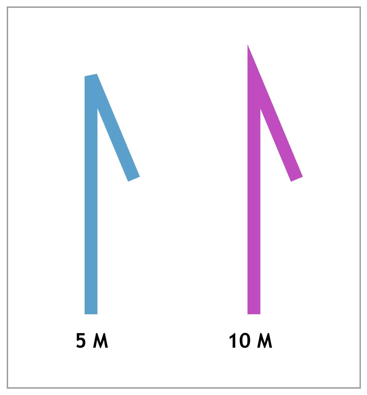
Figure 17: Forcing a beveled corner with 5 M

Increasing the miter limit from 5 M to 10 M will allow the PDF to display a sharp corner.

The cm Operator

Much like the Tm operator, cm sets the transformation matrix for everything drawn onto a page. Like the Tm matrix, it can rotate, scale, and skew graphics. But its most common usage is to change the origin of the page:

This stream starts by moving the origin to the center of the page (instead of the lower-left corner). Then it draws the exact same graphic as the previous section, but using coordinates that are relative to the new origin.

The q and Q Operators

Complex graphics are often built up from smaller graphics that all have their own state. It’s possible to separate elements from each other by placing operators in a q/Q block:

Everything between the q and Q operators happens in an isolated environment. As soon as Q is called, the cm operator is forgotten, and the origin returns to the bottom-left corner.

The RG, rg, K, and k Operators

While colors aren’t technically considered graphics state operators, they do determine the color of all future drawing operators, so this is a logical place to introduce them.

PDFs can represent several color spaces, the most common of which are RGB and CMYK. In addition, stroke color and fill color can be selected independently. This gives us four operators for selecting colors:

• RG: Change the stroke color space to RGB and set the stroke color.
• rg: Change the fill color space to RGB and set the fill color.
• K: Change the stroke color space to CMYK and set the stroke color.
• k: Change the fill color space to CMYK and set the fill color.

RGB colors are defined as a percentage between 0 and 1 for the red, green, and blue components, respectively. For example, the following defines a red stroke with a blue fill.

Likewise, the CMYK operators take four percentages, one each for cyan, magenta, yellow, and black. The previous stream makes use of the B operator, which strokes and fills the path.

Path Construction Operators

Setting the graphics state is like choosing a paintbrush and loading it with paint. The next step is to draw the graphics onto the page. However, instead of a putting a physical paintbrush to the page, we must represent graphics as numerical paths.

PDF path capabilities are surprisingly few:

• <x> <y> m: Move the cursor to the specified point.
• <x> <y> l: Draw a line from the current position to the specified point.
• <x1> <y1> <x2> <y2> <x3> <y3> c: Append a cubic Bézier curve to the current path.
• h: Close the current path with a line segment from the current position to the start of the path.

The m Operator

The m operator moves the graphics cursor (the “paintbrush”) to the specified location on the page. This is a very important operation—without it, all path segments would be connected and would begin at the origin.

The l (lowercase L) Operator

The l operator draws a line from the current point to another point. We’ve seen this many times in previous sections.

Remember that PDF is a low-level representation of text and graphics, so there is no “underlined text” in a PDF document. There is only text, and lines (as entirely independent entities). Underlining text must be performed manually.

The c Operator

This operator creates a cubic Bézier curve, which is one of the most common ways to represent complex vector graphics. A cubic Bézier curve is defined by four points:

Figure 18: An exemplary Bézier curve

If you’ve ever used the pen tool in Adobe Illustrator, you should be familiar with Bézier curves. The curve shown in the previous figure can be created in a PDF with the following stream.

The first anchor point is the current position (250, 250), the first control point is (300, 400), the second control point is (450, 450), and the final anchor is (550, 250).

The h Operator

The h operator closes the current path using a line segment from the current point to the beginning of the path. It takes no arguments. This operator can often be omitted, since many painting operators will automatically close the current path before painting it.

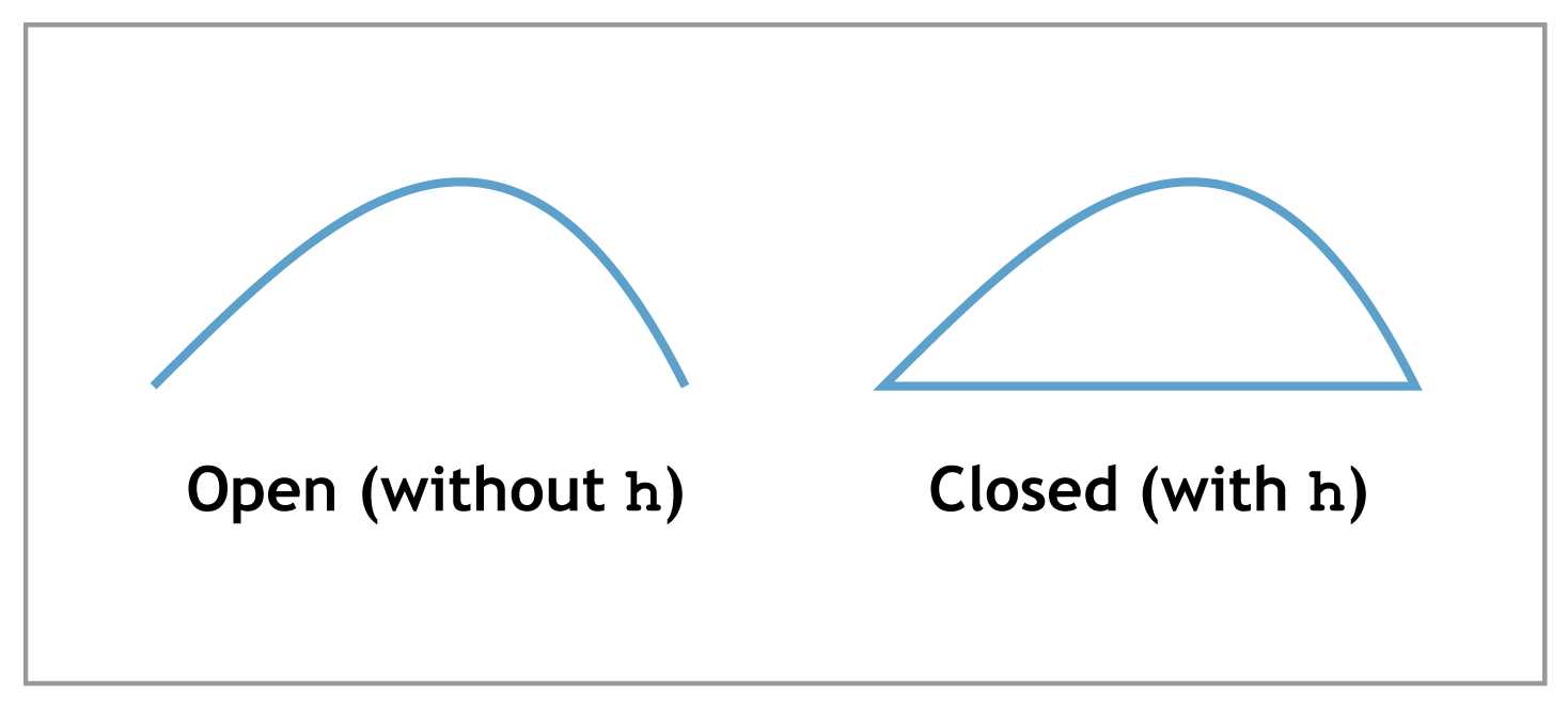
Figure 19: Closing the constructed path with the h operator

m, l, c, and h are the four main construction operators in a PDF. Again, there are no “shape” operators in the PDF specification—you cannot create a “circle” or a “triangle.” However, all shapes can be approximated as a series of lines, Bézier curves, or both. It is up to the PDF editor application to make higher-level shapes available to document authors and to transform them into a sequence of these simple construction operations.

Graphics Painting Operators

Once you’re done constructing a path, you must explicitly draw it with one of the painting operators. This is similar to the Tj operator for drawing text. After a painting operator is applied, the constructed path is finished—no more painting operators can be applied to it, and another call to a construction operator will begin a new path.

The S and s Operators

The S and s operators paint the stroke of the constructed path using the stroke width set by w and the stroke color set by RG or K. Before applying a stroke to the path, the lowercase version closes the current path with a line segment. This is the exact same behavior as h S.

The f Operator

The f operator fills the constructed path with the current fill color set by rg or k. The current path must be closed before painting the fill, so there is no equivalent to the capital S for painting strokes. The following stream creates a blue triangle.

Remember that painting a path completes the current path. This means the sequence f S will only fill the path—the S applies to a new path that has not been constructed yet. To fill and stroke a path, we need a dedicated operator.

The B and b Operators

The B and b operators paint and stroke the current path. Like s, the lowercase b closes the path before painting it. However, since filling a path implicitly closes it, the distinction between B and b can only be seen in the stroke as shown in the following figure.

Figure 20: Deciding to open or close a path via a painting operator

The * (asterisk) Operators

The fill behavior of f, B, and b are relatively straightforward for simple shapes. Painting fills becomes more complicated when you start working with paths that intersect themselves. For example, consider the following:

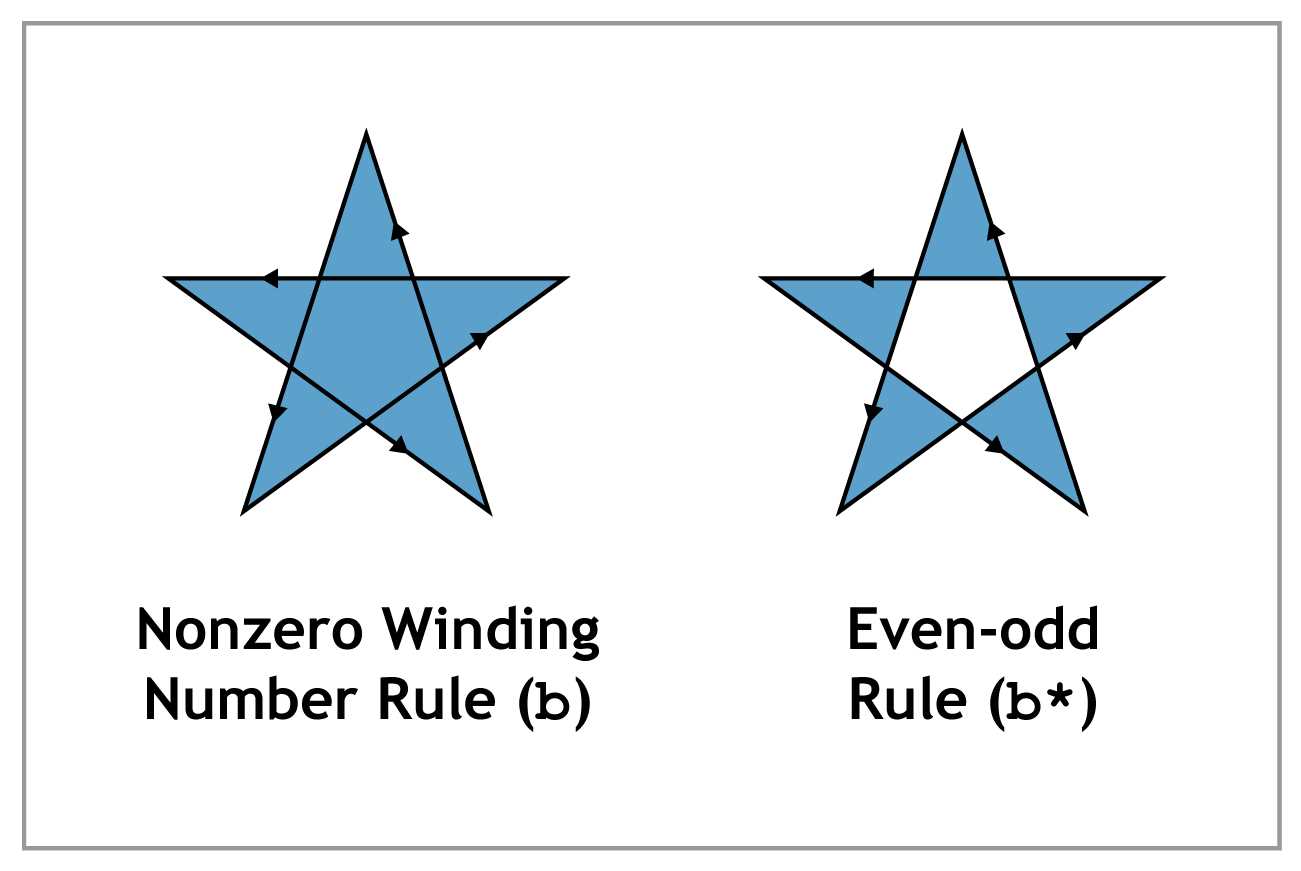
Figure 21: PDF’s fill algorithms

As you can see, such a path can be filled using two different methods: the nonzero winding number rule or the even-odd rule. The technical details of these algorithms are outside the scope of this book, but their effect is readily apparent in the previous diagram.

The fill operators we’ve seen thus far use the nonzero winding number rule. PDFs have dedicated operators for even-odd rule fills: f*, B*, and b*. Aside from the fill algorithm, these operators work the exact same as their un-asterisked counterparts.

Summary

PDFs were initially designed to be a digital representation of physical paper and ink. The graphics operators presented in this chapter make it possible to represent arbitrary paths as a sequence of lines and curves.

Like their textual counterparts, graphics operators are procedural. They mimic the actions an artist would take to draw the same image. This can be intuitive if you’re creating graphics from scratch, but can become quite complicated if you’re trying to manually edit an image. For example, it’s easy to say something like, “Draw a line from here to there,” but it’s much harder to say, “Move this box two inches to the left.” Once again, this task is left up to PDF editor applications.