Training

---

Introduction

The ultimate goal of a neural network is to make a prediction. In order to make a prediction, a neural network must first be trained. Training a neural network is the process of finding a set of good weights and bias values so that the known outputs of some training data match the outputs computed using the weights and bias values. The resulting weights and bias values for a particular problem are often collectively called a model. The model can then be used to predict the output for previously unseen inputs that do not have known output values.

Figure 5-a: Training Demo

To get a good feel for exactly what neural network training is, take a look at the screenshot of a demo program in Figure 5-a. The demo program solves a simple, but what is probably the most famous, problem in the field of neural networks. The goal is to predict the species of an iris flower from four numeric attributes of the flower: petal length, petal width, sepal length, and sepal width. The petal is what most people would consider the actual flower part of the iris. The sepal is a green structure that you can think of as a specialized leaf. There are three possible species: Iris setosa, Iris versicolor, and Iris virginica. The data set was first published in 1936 by mathematician Ronald Fisher and so it is often called Fisher's Iris data.

The data set consists of a total of 150 items, with data for 50 of each of the three species of iris. Because neural networks only understand numeric data, the demo must use data where the three possible y-values have been encoded as numbers. Here the species Iris sestosa is encoded as (0, 0, 1), Iris versicolor is encoded as (0, 1, 0), and the species Iris virginica is encoded as (1, 0, 0).

The demo takes the 150-item data set and splits it randomly into a 120-item subset (80%) to be used for training and a 30-item subset (20%) to be used for testing, that is, to be used to estimate the probability of a correct classification on data that has not been seen before. The demo trains a 4-7-2 fully connected neural network using the back-propagation algorithm in conjunction with a technique that is called incremental training.

After training has completed, the accuracy of the resulting model is computed on the training set and on the test set. The model correctly predicts 97.50% of the training items (117 out of 120) and 96.67% of the test items (29 out of 30). Therefore, if presented with data for a new iris flower that was not part of the training or test data, you could estimate that the model would correctly classify the flower with roughly a 0.9667 probability.

Incremental Training

There are two main approaches for training a neural network. As usual, the two approaches have several different names but two of the most common terms are incremental and batch. In high-level pseudo-code, batch training is:

loop until done
  for each training item
    compute error and accumulate total error
  end for
  use total error to update weights and bias values
end loop

The essence of batch training is that an error metric for the entire training set is computed and then that single error value is used to update all the neural network's weights and biases.

In pseudo-code, incremental training is:

loop until done
  for each training item
    compute error for current item
    use item's error to update weights and bias values
  end for
end loop

In incremental training, weights and biases are updated for every training item. Based on my conversations, to most people, batch training seems a bit more logical. However, some research evidence suggests that incremental training (also called online training) often gives better results (meaning it produces a model that predicts better) than batch training.

There is a third approach to neural network training, which is a combination of batch and incremental training. The technique is often called mini-batch training. In pseudo-code:

loop until done
  loop n times
    compute error term for current item
    accumulate error
  end loop
  use current accumulated error to update weights and bias values
  reset mini accumulated error to 0
end loop

The demo program uses incremental training. Notice that in all three training approaches there are two important questions: “How do you determine when training is finished?” and “How do you measure error?” To answer briefly, before the demo code is presented, there is no one best way to determine when training is done. There are two good ways to compute error.

Implementing the Training Demo Program

To create the demo program I launched Visual Studio and created a new C# console application named Training. After the template code loaded into the editor, I removed all using statements except for the single statement referencing the top-level System namespace. The demo program has no significant .NET version dependencies, so any version of Visual Studio should work. In the Solution Explorer window, I renamed file Program.cs to TrainingProgram.cs and Visual Studio automatically renamed the Program class to TrainingProgram.

The overall structure of the demo program is shown in Listing 5-a. The Main method in the program class has all the program logic. The program class houses three utility methods: MakeTrainTest, ShowVector, and ShowMatrix. Method ShowMatrix is used by the demo program to display the source data set, which is a matrix in memory, and the training and test matrices. The helper is defined:

static void ShowMatrix(double[][] matrix, int numRows, int decimals, bool newLine)

{

  for (int i = 0; i < numRows; ++i)

  {

    Console.Write(i.ToString().PadLeft(3) + ": ");

    for (int j = 0; j < matrix[i].Length; ++j)

    {

      if (matrix[i][j] >= 0.0) Console.Write(" "); else Console.Write("-");

      Console.Write(Math.Abs(matrix[i][j]).ToString("F" + decimals) + " ");

    }

    Console.WriteLine("");

  }

  if (newLine == true)

    Console.WriteLine("");

}

Listing 5-a: Overall Demo Program Structure

The numRows parameter to ShowMatrix controls how many rows of the matrix parameter to display, not the total number of rows in the matrix. The method displays row numbers and has a hard-coded column width of 3 for the line numbers. You may want to parameterize whether or not to display row numbers and use the actual number of matrix rows to parameterize the width for line numbers.

The method uses an if-check to determine if the current cell value is positive or zero, and if so, prints a blank space for the implicit "+" sign so that positive values will line up with negative values that have an explicit "-" sign. An alternative is to pass a conditional formatting string argument to the ToString method.

Helper method ShowVector is used by the demo to display the neural network weights and bias values after training has been performed. It is defined:

static void ShowVector(double[] vector, int valsPerRow, int decimals, bool newLine)

{

  for (int i = 0; i < vector.Length; ++i)

  {

    if (i % valsPerRow == 0) Console.WriteLine("");

    Console.Write(vector[i].ToString("F" + decimals).PadLeft(decimals + 4) + " ");

  }

  if (newLine == true)

    Console.WriteLine("");

}

Creating Training and Test Data

One of the strategies used in neural network training is called hold-out validation. This means to take the available training data, and rather than train the neural network using all the data, remove a portion of the data, typically between 10–30%, to be used to estimate the effectiveness of the trained model. The remaining part of the available data is used for training.

Method MakeTrainTest accepts a matrix of data and returns two matrices. The first return matrix holds a random 80% of the data items and the other matrix is one that holds the other 20% of the data items

In high-level pseudo-code, method MakeTrainTest is:

compute number of rows for train matrix := n1
compute number of rows for test matrix := n2
make a copy of the source matrix
scramble the order of the rows of the copy
copy first n1 rows of scrambled-order source copy into train
copy remaining n2 rows of scrambled-order source copy into test
return train and test matrices

The implementation of method MakeTrainTest begins:

static void MakeTrainTest(double[][] allData, int seed,

  out double[][] trainData, out double[][] testData)

{

  Random rnd = new Random(seed);

The method accepts a data matrix to split, and a seed value to initialize the randomization process. The method returns the resulting train and test matrices as out parameters. Although returning multiple results via out parameters is frowned upon in certain circles, in my opinion using this approach is simpler than alternative designs such as using a container class.

Because method MakeTrainTest is called only once in the demo program, it is acceptable to use a Random object with local scope. If the method were called multiple times, the results would be the same unless you passed different seed parameter values on each call.

Next, the method allocates space for the two return matrices like so:

int totRows = allData.Length;

int numCols = allData[0].Length;

int trainRows = (int)(totRows * 0.80); // Hard-coded 80-20 split.

int testRows = totRows - trainRows;

trainData = new double[trainRows][];

testData = new double[testRows][];

Notice that the method is hard-coded for an 80-20 train-test split. You might want to consider passing the training size as a parameter. This can be tricky because percentages might be in decimal form, such as 0.80, or in percentage form, such as 80.0. Notice that because of possible rounding, it would be risky to compute the number of result rows with code like this:

int trainRows = (int)(totRows * 0.80); // risky

int testRows = (int)(totRows * 0.20);

Next, method MakeTrainTest makes a reference copy of the source matrix:

double[][] copy = new double[allData.Length][];

for (int i = 0; i < copy.Length; ++i)

  copy[i] = allData[i];

This code is a bit subtle. Instead of making a copy of the source matrix, it would be perfectly possible to operate directly on the matrix. However this would have the side effect of scrambling the order of the source matrix's rows. The copy of the source matrix is a reference copy. The diagram in Figure 5-b shows what a copy of a source matrix with nine rows of data would look like in memory. It would be possible to make a complete copy of the source matrix’s values but this would be inefficient and might not even be feasible if the source matrix were very large.

Next the reference copy is randomized:

for (int i = 0; i < copy.Length; ++i)

{

  int r = rnd.Next(i, copy.Length);

  double[] tmp = copy[r];

  copy[r] = copy[i];

  copy[i] = tmp;

}

The rows of the copy matrix are scrambled using the Fisher-Yates shuffle algorithm which randomly reorders the values in an array. In this case, the values are references to the rows of the copy matrix. The Fisher-Yates shuffle is also quite subtle, but after the code executes, the copy matrix will have the same values as the source but the rows will be in a random order.

Method MakeTrainTest continues by copying rows of the scrambled copy matrix into the trainData result matrix:

for (int i = 0; i < trainRows; ++i)

{

  trainData[i] = new double[numCols];

  for (int j = 0; j < numCols; ++j)

  {

    trainData[i][j] = copy[i][j];

  }

}

Notice the copy-loop allocates space for the result matrix rows. An alternative would be to perform the allocation in a separate loop.

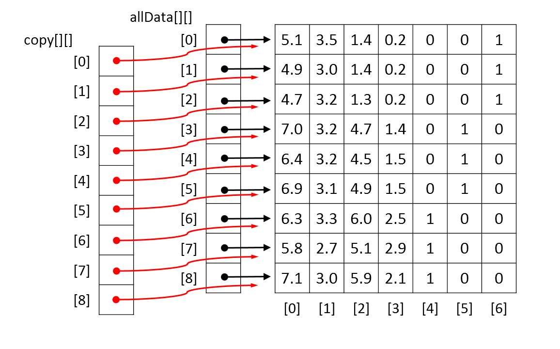
Figure 5-b: Copying a Matrix by Reference

Method MakeTrainTest concludes by copying rows of the scrambled copy matrix into the testData result matrix:

  for (int i = 0; i < testRows; ++i) // i points into testData[][]

  {

    testData[i] = new double[numCols];

    for (int j = 0; j < numCols; ++j)

    {

      testData[i][j] = copy[i + trainRows][j]; // be careful

    }

  }

} // MakeTrainTest

In this code, variable trainRows will be 120 and testRows will be 30. Row index i points into the testData result matrix and runs from 0 through 29. In the copy assignment, the value i + trainRows points into the source copy matrix and will run from 0 + 120 = 120 through 29 + 120 = 149.

The Main Program Logic

After some preliminary WriteLine statements, the Main method sets up the iris data:

static void Main(string[] args)

{

  // Preliminary messages.

  double[][] allData = new double[150][];

  allData[0] = new double[] { 5.1, 3.5, 1.4, 0.2, 0, 0, 1 };
  . . .

  allData[149] = new double[] { 5.9, 3.0, 5.1, 1.8, 1, 0, 0 };

For simplicity, the data is placed directly into an array-of-arrays style matrix. Notice the y-data to classify has been pre-encoded as (0, 0, 1), (0, 1, 0), and (1, 0, 0), and that there is an implicit assumption that the y-data occupies the rightmost columns of the matrix. Also, because the x-data values all have roughly the same magnitude, there is no need for data normalization.

In most situations, your data would be in external storage, such as a text file. For example, suppose the demo data were stored in a text file named IrisData.txt with this format:

5.1,3.5,1.4,0.2,0,0,1
4.9,3.0,1.4,0.2,0,0,1
. . .
5.9,3.0,5.1,1.8,1,0,0

One possible implementation of a method named LoadData to load the data into a matrix is presented in Listing 5-b. The method could be called along the lines of:

string dataFile = "..\\..\\IrisData.txt";

allData = LoadData(dataFile, 150, 7);

In situations where the source data is too large to fit into a matrix in memory, the simplest approach is to stream through the external data source. A complicated alternative is to buffer the streamed data through a matrix.

After loading the data into memory, the Main method displays the first six rows of the data matrix like so:

Console.WriteLine("\nFirst 6 rows of the 150-item data set:");

ShowMatrix(allData, 6, 1, true);

Next, the demo creates training and test matrices:

Console.WriteLine("Creating 80% training and 20% test data matrices");

double[][] trainData = null;

double[][] testData = null;

MakeTrainTest(allData, 72, out trainData, out testData);

The rather mysterious looking 72 argument is the seed value passed to the Random object used by method MakeTrainTest. That value was used only because it gave a representative, and pretty, demo output. In most cases you would simply use 0 as the seed value.

Listing 5-b: Loading Data from a File

The main program logic continues by displaying portions of the newly created training and test data matrices:

Console.WriteLine("\nFirst 3 rows of training data:");

ShowMatrix(trainData, 3, 1, true);

Console.WriteLine("First 3 rows of test data:");

ShowMatrix(testData, 3, 1, true);

Of course such displays are purely optional when working with neural networks but are often extremely useful during development in order to catch errors early. Total control over your system, including the ability to insert diagnostic display messages anywhere in the system, is a big advantage of writing custom neural network code versus using a packaged system or API library written by someone else.

After creating the training and test matrices, method Main instantiates a neural network:

Console.WriteLine("\nCreating a 4-input, 7-hidden, 3-output neural network");

Console.Write("Hard-coded tanh function for input-to-hidden and softmax for ");

Console.WriteLine("hidden-to-output activations");

int numInput = 4;

int numHidden = 7;

int numOutput = 3;

NeuralNetwork nn = new NeuralNetwork(numInput, numHidden, numOutput);

The number of input nodes and the number of output nodes are determined by the structure of the source data: four numeric x-values and a y-value with three categorical values. Specifying a good value for the number of hidden nodes is one of the major challenges when working with neural networks. Even though there has been much research done in this area, picking a good value for the number of hidden nodes is mostly a matter of trial and error.

With the data prepared and a neural network instantiated, the Main method performs training like so:

int maxEpochs = 1000;

double learnRate = 0.05;

double momentum = 0.01;

Console.WriteLine("Setting maxEpochs = " + maxEpochs + ", learnRate = " +

  learnRate + ", momentum = " + momentum);

Console.WriteLine("Training has hard-coded mean squared " +

  "error < 0.040 stopping condition");

Console.WriteLine("\nBeginning training using incremental back-propagation\n");

nn.Train(trainData, maxEpochs, learnRate, momentum);

Console.WriteLine("Training complete");

The maxEpochs variable sets a hard limit on the number of iterations that will be performed in the training code. As you will see shortly, it is not trivial to determine when to stop the main training loop. The learningRate and momentum values control the speed at which the back-propagation converges to a final set of weight and bias values. As it turns out, back-propagation is extremely sensitive to the values used for the learning rate and momentum. Even small changes in these value can have very large effects and can mean the difference between a neural network that predicts well and one that predicts poorly.

For simplicity, the demo neural network has a fourth parameter, an early-exit error threshold value of 0.040 that is hard-coded into method Train. In many situations you would want to parameterize this value along the lines of:

int maxEpochs = 1000;

double learnRate = 0.05;

double momentum = 0.01;
double exitError = 0.040;
nn.Train(trainData, maxEpochs, learnRate, momentum, exitError);

After training has completed, the demo retrieves and displays the internal weights and bias values that were determined by the training process:

double[] weights = nn.GetWeights();

Console.WriteLine("Final neural network weights and bias values:");

ShowVector(weights, 10, 3, true);

The Main method concludes by computing and displaying the accuracy of the generated model:

  double trainAcc = nn.Accuracy(trainData);

  Console.WriteLine("\nAccuracy on training data = " + trainAcc.ToString("F4"));

  double testAcc = nn.Accuracy(testData);

  Console.WriteLine("\nAccuracy on test data = " + testAcc.ToString("F4"));

  Console.WriteLine("\nEnd neural network training demo\n");

  Console.ReadLine()

} // Main

Notice that the accuracy of the neural network on the training data was not used as a condition for stopping training, and is computed only after training has completed. The accuracy of the model on the test data is the more important of the two accuracy metrics. The accuracy of the model on the test data gives you a rough estimate of the accuracy of the model on new data with unknown y-values. A high accuracy on the training data does not necessarily indicate a good model has been generated, but a low accuracy on the test data almost always indicates a poor model.

Training and Error

Method Train is presented in Listing 5-c. Although the method is relatively short, it contains several important ideas that must be understood in order for you to be able to modify the code to meet specific problem scenarios.

Listing 5-c: Training a Neural Network

The heart of method Train is a while loop that has two exit conditions. The first is a hard limit based on the maxEpochs value. The second exit condition is a small error threshold based on the mean squared error of the current model over the entire training set. Inside the primary outer while-loop is a for-loop that iterates over each item in the training data. The local array named sequence and helper method Shuffle act to make the inner loop visit each training item in a different, random order, each time through the outer loop.

Visiting the training items in a random order is extremely important. Failure to visit training items in a random order is a common mistake and often leads to the training process quickly converging to a poor set of weights and bias values. The key to visiting data items in random order is helper method Shuffle:

private static void Shuffle(int[] sequence)

{

  for (int i = 0; i < sequence.Length; ++i)

  {

    int r = rnd.Next(i, sequence.Length);

    int tmp = sequence[r];

    sequence[r] = sequence[i];

    sequence[i] = tmp;

  }

}

Method Shuffle accepts an array of array indices and scrambles the order of the indices using the Fisher-Yates algorithm. For example, if a tiny training matrix had just four rows of data and the input parameter array named sequence held values { 0, 1, 2, 3 } then after a call to Shuffle, the values could be { 3, 0, 1, 2 } or any one of the 23 other possible permutations of the ordering.

In the inner for-loop in method Train, index variable i points into the array named sequence and index variable idx points into the rows of the training data matrix. For example, for a four-item training set, if array sequence holds values { 3, 0, 1, 2 } then index variable i takes on values 0, 1, 2, 3; and index variable idx takes on values 3, 0, 1, 2, which is the order in which the training data items would be visited. Notice that the array named sequence needs to be initialized only once, outside the outer while-loop in method Train.

An alternative to the shuffling technique presented here is instead of generating an array of row indices and shuffling the order of the values in that array, actually shuffling the order of the rows of the training data matrix. This would use slightly less memory (no sequence array needed) and have slightly better performance (no assignment to variable idx needed) at the expense of having a side effect (changing the order of the rows of the training data matrix).

The primary training loop in method Train exits when one of two conditions occur: the maximum number of iterations stored in variable maxEpochs is reached, or when the mean squared error drops below a hard-coded 0.040 value. Understanding and modifying the training-loop exit is one of the most important features of working with neural networks.

At first thought, it would seem that a reasonable strategy would be to simply train a neural network for as many iterations as possible. This approach often leads to over-fitting, a situation where the resulting model's weight and bias values fit the training data very well (often nearly perfectly) but when presented with new data, the model predicts very poorly.

The technique used by the demo is to use a moderate number for the hard-stop loop exit combined with the mean squared error (MSE). MSE is perhaps best explained by example. Suppose a mini training set of iris flower data consisted of just two training items:

5.0, 3.0, 1.5, 0.5, 0, 0, 1
6.0, 3.5, 1.7, 0.4, 0, 1, 0

Now suppose that for a given set of weights and bias values, the computed outputs for the two data items are (0.2, 0.1, 0.7) and (0.3, 0.6, 0.1) respectively. The squared error for the first training data item is (0 - 0.2)² + (0 - 0.1)² + (1 - 0.7)² = 0.04 + 0.01 + 0.09 = 0.14. The squared error for the second training data item is (0 - 0.3)² + (1 - 0.6)² + (0 - 0.1)² = 0.09 + 0.16 + 0.01 = 0.26. The total squared error of the mini training data set is 0.14 + 0.26 = 0.40. So, the mean (average) squared error, MSE, for the two items is 0.40 / 2 = 0.20.

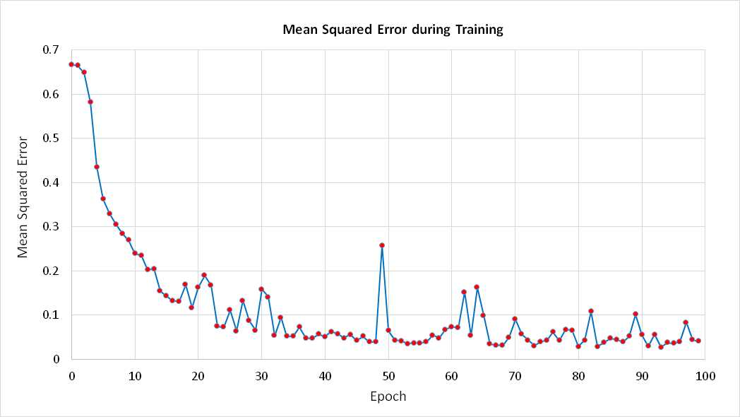
Figure 5-c: Mean Squared Error

A common approach to terminating training is to exit when the MSE drops below some threshold. This is the technique used by the demo program. Although reasonable, the approach does have a weakness. Typically, during neural network training, the MSE does not decrease in a completely smooth, monotonic manner. Instead, the MSE jumps around a bit. For example, the graph in Figure 5-c shows how MSE changes over time for the demo program. The data was generated simply by inserting this statement inside the outer while-loop in method Train:

Console.WriteLine(epoch + " " + mse.ToString("F4"));

Suppose the early-exit MSE threshold value were set to 0.15 (an artificially large value). If you examine the graph between epochs 10 and 30 closely, you can see that the MSE drops below 0.15 at epoch 15. However, the MSE jumps above 0.15 at epoch 20. The point is that using a single MSE exit threshold value is simple and usually effective, but runs the risk of stopping training too early.

One interesting approach to the loop-exit issue is to divide all available data into three sets rather than just training and test sets. The third set is called the validation set. For example, using a 60-20-20 split for the 150-item Fisher's Iris data, 90 items (60% of 150) would be in the training set, 30 items (20% of 150) would be in the test set, and the remaining 30 items would be in the validation set.

You would train the neural network using the training data, but inside the main training loop you would compute the MSE on the validation set. Over time the MSE on the validation set would drop but at some point, when over-fitting begins to occur, the MSE on the validation set would begin to increase. You would identify at what epoch the MSE on the validation set began to steadily increase (either programmatically or visually by graphing MSE) and then use the weights and bias values at that epoch for the final neural network model. And then you would compute the accuracy of the model on the unused test data set to get an estimate of the model's accuracy for new data.

Helper method MeanSquaredError is presented in Listing 5-d. Notice that in both method Train and in method MeanSquaredError, arrays xValues and tValues are used to store the values of the current input values and target values, and that the values are copied in by value rather than reference from the training data matrix. This is simple and effective but somewhat inefficient. An alternative is to make copies by reference.

Also notice that in all methods of the demo program, there is an implicit assumption that the encoded y-values occupy the last numOutput columns of the training matrix. When working with neural networks, there is no standard way to store data internally. The encoded y-values can be stored in the last columns of a training matrix as in the demo program, in the first columns, or the x-values and y-values can be stored in separate matrices. How to store training data is an important design decision and one that affects the code in many of the methods used during training.

Listing 5-d: Computing Mean Squared Error

The MSE value is an average error per training item and so an error-exit threshold value does not depend on the number of training items there are. However, if you refer back to how MSE is computed, you can see that MSE does depend to some extent on the number of possible classes there are in the y-data. Therefore, an alternative to using a fixed MSE threshold is to use a value that is based on the number of output values, for example 0.005 * numOutput.

Method Train computes and checks the MSE value on every iteration through the training loop. Computing MSE is a relatively expensive operation, so an alternative is to compute MSE only every 10 or 100 or 1,000 iterations along the lines of:

if (epoch % 100 == 0)

{

  double mse = MeanSquaredError(trainData);

  if (mse < 0.040) break;

}

Computing Accuracy

The code for public class method Accuracy is presented in Listing 5-e. How method Accuracy works is best explained using a concrete example. Suppose the computed output values and the desired target values for three training items are:

0.2  0.1  0.7   0  0  1
0.1  0.6  0.3   0  1  0
0.4  0.5  0.1   1  0  0

For the first data item, the three computed output values of 0.2, 0.1, and 0.7 can be loosely interpreted to mean the probabilities of the three possible categorical y-values. The demo program uses a technique called winner-takes-all. The idea is to find the highest probability, in this case 0.7, and then check the associated desired target value to see if it is 1 (a correct prediction) or 0 (an incorrect prediction). Because the third target output is a 1, the first data item was correctly predicted.

Listing 5-e: Computing Model Accuracy

For the second data item, the largest computed output is 0.6 which is in the second position, which corresponds to a target value of 1, so the second data item is also a correct prediction.

For the third data item, the largest computed output is 0.5. The associated target value is 0, so the third data item is an incorrect prediction.

Method Accuracy uses a helper method MaxIndex to find the location of the largest computed y-value. The helper is defined:

private static int MaxIndex(double[] vector)

{

  int bigIndex = 0;

  double biggestVal = vector[0];

  for (int i = 0; i < vector.Length; ++i)

  {

    if (vector[i] > biggestVal)

    {

      biggestVal = vector[i];

      bigIndex = i;

    }

  }

  return bigIndex;

}

Notice that method MaxIndex does not take into account the possibility that there may be two or more computed y-values that have equal magnitude. In practice this is usually not a problem, but for a neural network that is part of some critical system you would want to handle this possibility at the expense of slightly slower performance.

Method Accuracy also has two implementation choices that you may want to modify depending on your particular problem scenario. First, the method does a check for exact equality between value tValues[maxIndex] and the constant value 1.0. Because many type double values are just extremely close approximations to their true values, a more robust approach would be to check if tVlaues[maxIndex] is within some very small value (typically called epsilon) of 1.0. For example:

if (Math.Abs(tValues[maxIndex] - 1.0) < 0.000000001)

  ++numCorrect;

In practice, checking for the exact equality of an array value and the constant 1.0 is usually not a problem. The second implementation issue in method Accuracy is that the computation of the return value does not perform a division by zero check. This could only happen if the quantity numCorrect + numWrong were equal to 0. The ability to deliberately take intelligent shortcuts like this to improve performance and reduce code complexity is a big advantage of writing custom neural network code for your own use.

At first thought, it might seem that instead of using some error metric such as MSE to determine when to stop training, it would be preferable to use the accuracy of the neural network on the training data using its current weight and bias values. After all, in the end, prediction accuracy, not error, is the most important characteristic of a neural network. However, using accuracy to determine when to stop training is not as effective as using error. For example, suppose a neural network, Model A, has computed and target output values:

0.1  0.2  0.7   0  0  1
0.1  0.8  0.1   0  1  0
0.3  0.3  0.4   1  0  0

Model A correctly predicts the first two data items but misses the third and so has a classification accuracy of 2/3 = 0.6667. The MSE for Model A is (0.14 + 0.06 + 0.74) / 3 = 0.3133.

Now consider a Model B with computed and target output values of:

0.3  0.3  0.4   0  0  1
0.3  0.4  0.3   0  1  0
0.1  0.1  0.8   1  0  0

Model B also predicts the first two data items correctly and so has a classification accuracy of 0.6667. But Model B is clearly worse than Model A. Model B just barely gets the first two items correct and misses badly on the third. The MSE for Model B is (0.54 + 0.54 + 1.46) / 3 = 0.8467 which is more than twice as large as the MSE for Model A. In short, classification accuracy is too coarse of a metric to use during training.

Cross Entropy Error

There is an important alternative to mean squared error called mean cross entropy error. There is some strong, but not entirely conclusive, research evidence to suggest that for many classification problems, using mean cross entropy error generates better models than using mean squared error. Exactly what cross entropy error is, is best explained by example. Suppose that for some neural network there are just two training items with three computed output values and three associated desired target output values:

0.1  0.2  0.7   0  0  1
0.3  0.6  0.1   0  1  0

The cross entropy error for the first data item is computed as:

- ( (ln(0.1) * 0) + (ln(0.2) * 0) + (ln(0.7) * 1) ) = - ( 0 + 0 + (-0.36) ) = 0.36

The cross entropy error for the second data item is:

- ( (ln(0.3) * 0) + (ln(0.6) * 1) + (ln(0.1) * 0) ) = - ( 0 + (-0.51) + 0 ) = 0.51

Here ln is the natural logarithm function. The mean (average) cross entropy error is (0.36 + 0.51) / 2 = 0.435. Notice the odd-looking multiplications by 0. This is a consequence of the mathematical definition of cross entropy error and the fact that for neural classification problems all target values except one will have value 0. One possible implementation of a mean cross entropy error function is presented in Listing 5-f.

Using mean cross entropy error is very deep mathematically but simple in practice. First, mean cross entropy error can be used as a training-loop exit condition in exactly the same way as mean squared error. The second way to use mean cross entropy error is during the back-propagation routine during training. In the demo program, method Train calls method ComputeOutputs to perform the feed-forward part of training and calls method UpdateWeights to modify all neural network weights and bias values using the back-propagation algorithm.

Listing 5-f: Mean Cross Entropy Error

As it turns out, the back-propagation algorithm is making an implicit assumption about what error metric is being used behind the scenes. This assumption is needed to compute a calculus derivative which in turn is implemented in code. Put another way, if you examine the code for the back-propagation algorithm inside method UpdateWeights you will not see an explicit error term being computed. The error term used is actually mean squared error but it is computed implicitly and has an effect when the gradient values for the hidden layer and output layer nodes are computed.

Therefore, if you want to use mean cross entropy error for neural network training, you need to know what the implicit effect on back-propagation in method UpdateWeights is. Inside method UpdateWeights, the implicit mean squared error code occurs in two places. The first is the computation of the output node gradient values. The computation of output gradients with an assumption of the standard MSE is:

for (int i = 0; i < numOutput; ++i)

{

  double derivative = (1 - outputs[i]) * outputs[i]; // Softmax activation.

  oGrads[i] = derivative * (tValues[i] - outputs[i]);

}

The computation of output gradients with an assumption of cross entropy error is rather amazing:

for (int i = 0; i < numOutput; ++i)

{

  oGrads[i] = tValues[i] - outputs[i]; // Assumes softmax.

}

In essence, the derivative term drops out altogether. Actually, the derivative is still computed when using cross entropy error but several terms cancel each other out leaving the remarkably simple result that the output gradient is just the target value minus the computed output value.

This result is one of the most surprising in neural networks. Because of the simplicity of the gradient term when using cross entropy error, it is sometimes said that cross entropy is the natural error term to use with neural network classification problems.

The second place where the implied error term emerges is in the computation of the hidden node gradient values. The hidden node gradient code which assumes MSE is:

for (int i = 0; i < numHidden; ++i)

{

  double derivative = (1 - hOutputs[i]) * (1 + hOutputs[i]); // tanh

  double sum = 0.0;

  for (int j = 0; j < numOutput; ++j)

  {

    double x = oGrads[j] * hoWeights[i][j];

    sum += x;

  }

  hGrads[i] = derivative * sum;

}

To modify this code so that it implicitly uses mean cross entropy error you would likely guess that the derivative term vanishes here too. However, again, somewhat surprisingly, this time the code does not change at all. You can find the elegant but complex mathematical derivations of the computation of back-propagation gradient values for both MSE and cross entropy error in many places on the Internet.

Binary Classification Problems

The iris data classification problem has three possible categorical y-values. Problems that have only two possible categorical y-values are very common. You can image predicting a person's sex (male or female) based on x-data like height, occupation, left or right hand dominance, and so on. Or consider predicting a person's credit worthiness (approve loan, reject loan) based on things like credit score, current debt, annual income, and so on.

Classification problems where the y-value to predict can be one of two values are called binary classification problems. Problems where there are three or more categorical y-values to predict are sometimes called multinomial classification problems to distinguish them from binary classification problems.

Dealing with a binary classification problem can in principle be done using the exact same techniques as those used for multinomial classification problems. For example, suppose the iris data file contained only data for two species, Iris setosa and Iris versicolor along the lines of:

5.1, 3.5, 1.4, 0.2, Iris-setosa
4.9, 3.0, 1.4, 0.2, Iris-setosa
. . .
5.7, 2.8, 4.1, 1.3, Iris-versicolor

You could encode the data like so:

5.1, 3.5, 1.4, 0.2, 0, 1
4.9, 3.0, 1.4, 0.2, 0, 1
. . .
5.7, 2.8, 4.1, 1.3, 1, 0

Here, Iris setosa is encoded as (0, 1) and Iris versicolor is encoded as (1, 0). Your neural network would have four input nodes and two output nodes. The network would use softmax activation on the output nodes and generate two computed outputs that sum to 1.0. For example, for the first data item in the previous example with target values of (0, 1), the computed output values might be (0.2, 0.8). In short, you would use the exact same technique for a binary problem as when there are three or more possible y-values.

However, binary classification problems can be encoded using a single value rather than two values. This is a consequence of the fact that, if you have two values that must sum to 1.0, and you know just one of the two values, you automatically know what the other value must be.

So, the previous data could be encoded as:

5.1, 3.5, 1.4, 0.2, 0
4.9, 3.0, 1.4, 0.2, 0
. . .
5.7, 2.8, 4.1, 1.3, 1

where Iris setosa is encoded as a 0 and Iris versicolor is encoded as a 1. If you encode using this 0-1 way, you must make two changes to the approach used by the demo program for multinomial classification.

First, when computing neural network output values, using softmax activation for the output layer nodes will not work because softmax assumes there are two or more nodes and coerces them to sum to 1.0. If you encode a binary classification problem using a 0-1 approach then you should use the logistic sigmoid function for output layer activation. For example, suppose you define the logistic sigmoid as:

public double LogSigmoid(double x)

{

  if (x < -45.0)

    return 0.0;

  else if (x > 45.0)

    return 1.0;

  else

    return 1.0 / (1.0 + Math.Exp(-x));

}

Then in method ComputeOutputs, the following lines of code:

double[] softOut = Softmax(oSums); // All outputs at once.

Array.Copy(softOut, outputs, softOut.Length);

would be replaced by this:

for (int i = 0; i < numOutput; ++i) // Single output node.

  outputs[i] = LogSigmoid(oSums[i]);

Because the logistic sigmoid function and the softmax function both have the same calculus derivatives, you do not need to make any changes to the back-propagation algorithm. And the hyperbolic tangent function remains a good choice for hidden layer activation for 0-1 encoded binary classification problems.

When using 0-1 encoding for a binary classification problem, the second change occurs in computing classification accuracy. Instead of finding the index of the largest computed output value and checking to see if the associated target value is 1.0, you just examine the single computed value and check to see if it is less than or equal to 0.5 (corresponding to a target y-value of 0) or greater than 0.5 (corresponding to a target y-value of 1).

For example, inside class method Accuracy, the code for softmax output is:

int maxIndex = MaxIndex(yValues); // Which cell in yValues has the largest value?

if (tValues[maxIndex] == 1.0)

  ++numCorrect;

else

  ++numWrong;

Those two statements would be replaced with:

if (yValues[0] <= 0.5 && tValues[0] == 0.0)

  ++numCorrect;

else if (yValues[0] > 0.5 && tValues[0] == 1.0)

  ++numCorrect;

else

  ++numWrong;

Notice that with 0-1 encoding both the tValues target outputs array and the yValues computed outputs array will have a length of just one cell and so are referenced by tValues[0] and yValues[0]. You could refactor all occurrences of the tValues and yValues arrays to simple variables of type double, but this would require a lot of work for no significant gain.

To recap, when working with a binary classification problem you can encode the first y-value as (0, 1), the second y-value as (1, 0), and use the exact same code as in the demo which works with multinomial classification. Or you can encode the first y-value as 0, the second y-value as 1, and make two changes to the demo neural network (in method ComputeOutputs and method Accuracy).

Among my colleagues, the vast majority prefer to use 0-1 encoding for binary classification problems. Their argument is that the alternative of using (0, 1) and (1, 0) encoding creates additional weights and biases that must be found during training. I prefer using (0, 1) and (1, 0) encoding for binary classification problems. My argument is that I only need a single code base for both binary and multinomial problems.

Complete Demo Program Source Code