Back-Propagation

---

Introduction

Back-propagation is an algorithm that can be used to train a neural network. Training a neural network is the process of finding a set of weights and bias values so that, for a given set of inputs, the outputs produced by the neural network are very close to some known target values. Once you have these weight and bias values, you can apply them to new input values where the output value is not known, and make a prediction. This chapter explains the back-propagation algorithm.

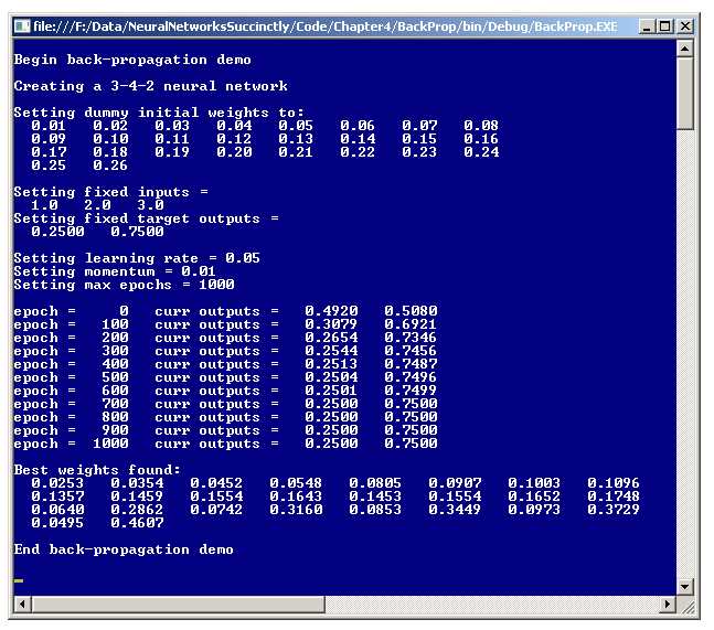
Figure 4-a: Back-Propagation Demo

There are alternatives to back-propagation (which is often spelled as the single word backpropagation), but back-propagation is by far the most common neural network training algorithm. A good way to get a feel for exactly what back-propagation is, is to examine the screenshot of a demo program shown in Figure 4-a. The demo program creates a dummy neural network with three inputs, four hidden nodes, and two outputs. The demo neural network does not correspond to a real problem and works on only a single data item.

The demo neural network has fixed, arbitrary input values of 1.0, 2.0, and 3.0. The goal of the demo program is to find a set of 26 weights and bias values so that the computed outputs are very close to arbitrary target output values of 0.2500 and 0.7500. Back-propagation is an iterative process. After 1,000 iterations, the demo program did in fact find a set of weight and bias values that generate output values which are very close to the two desired target values.

Back-propagation compares neural network computed outputs (for a given set of inputs, and weights and bias values) with target values, determines the magnitude and direction of the difference between actual and target values, and then adjusts the neural network's weights and bias values so that the new outputs will be closer to the target values. This process is repeated until the actual output values are close enough to the target values, or some maximum number of iterations has been reached.

The Basic Algorithm

There are many variations of the back-propagation algorithm. Expressed in high-level pseudo-code, basic back-propagation is:

loop until some exit condition
  compute output values
  compute gradients of output nodes
  compute gradients of hidden layer nodes
  update all weights and bias values
end loop

Gradients are values that reflect the difference between a neural network's computed output values and the desired target values. As it turns out, gradients use the calculus derivative of the associated activation function. The gradients of the output nodes must be computed before the gradients of the hidden layer nodes, or in other words, in the opposite direction of the feed-forward mechanism. This is why back-propagation, which is a shortened form of "backwards propagation", is named as it is. Unlike gradients which must be computed in a particular order, the output node weights and biases and the hidden layer node weights and biases can be updated in any order.

If you refer to the screenshot in Figure 4-a, you can see that back-propagation uses a learning rate parameter and a momentum parameter. Both of these values influence how quickly back-propagation converges to a good set of weights and bias values. Large values allow back-propagation to learn more quickly but at the risk of overshooting an optimal set of values. Determining good values for the learning rate and the momentum term is mostly a matter of trial and error. The learning rate and momentum term are called free parameters; you are free to set their values to whatever you choose. Weights and biases are also called free parameters.

Many neural network references state that back-propagation is a simple algorithm. This is only partially true. Once understood, back-propagation is relatively simple to implement in code. However, the algorithm itself is very deep. It took machine learning researchers many years to derive the basic back-propagation algorithm.

Computing Gradients

The first step in the back-propagation is to compute the values of the gradients for the output nodes. Figure 4-b represents the dummy 3-4-2 neural network of the demo program. The three fixed input values are 1.0, 2.0, and 3.0. The 26 weights and bias values are 0.01, 0.02, . . 0.26.

The current output values generated by the inputs and weights and bias values are 0.4920 and 0.5080. The neural network is using the hyperbolic tangent function for the hidden layer nodes and softmax activation for output layer nodes. The desired target values are 0.2500 and 0.7500.

Figure 4-b: The Back-Propagation Mechanism

The gradient of an output node is the difference between the computed output value and the desired value, multiplied by the calculus derivative of the activation function used by the output layer. The difference term is reasonable but exactly why the calculus derivative term is used is not at all obvious and is a result of deep but beautiful mathematics.

The calculus derivative of the softmax activation function at some value y is just y(1 - y). Again, this is not obvious and is part of the mathematics of neural networks. The values of the output node gradients are calculated as:

oGrad[0] = (1 - 0.4920)(0.4920) * (0.2500 - 0.4920) = 0.2499 * -0.2420 = -0.0605 (rounded)
oGrad[1] = (1 - 0.5080)(0.5080) * (0.7500 - 0.5080) = 0.2499 * 0.2420 = 0.0605

The first part of the computation is the derivative term. The second part is the difference between computed and desired output values. The order in which the difference between computed and desired values is performed is very important but varies from implementation to implementation. Here, the difference is computed as (desired - computed) rather than (computed - desired).

Computing the values of the hidden node gradients uses the values of the output node gradients. The gradient of a hidden node is the derivative of its activation function times the sum of the products of "downstream" (to the right in Figure 4-b) output gradients and associated hidden-to-output weights. Note that computing gradient values in the way described here makes an implicit mathematical assumption about exactly how error is computed.

The calculation is best explained by example. As it turns out, the derivative of the hyperbolic tangent at some value y is (1 - y)(1 + y). The gradient for hidden node 0, with rounding, is computed as:

hGrad[0]:
  derivative = (1 - 0.4699)(1 + 0.4699) = 0.5301 * 1.4699 = 0.7792
  sum = (-0.0605)(0.17) + (0.0605)(0.18) = -0.0103 + 0.0109 = 0.0006
  hGrad[0] = 0.7792 * 0.0006 = 0.00047 (rounded)

Similarly, the gradient for hidden node 1 is:

hGrad[1]:
  derivative = (1 - 0.5227)(1 + 0.5227) = 0.4773 * 1.5227 = 0.7268
  sum = (-0.0605)(0.19) + (0.0605)(0.20) = -0.0115 + 0.0121 = 0.0006
  hGrad[3] = 0.7268 * 0.0006 = 0.00044

And:

hGrad[2]:
  derivative = (1 - 0.5717)(1 + 0.5717) = 0.4283 * 1.5717= 0.6732
  sum = (-0.0605)(0.21) + (0.0605)(0.22) = -0.0127 + 0.0133 = 0.0006
  hGrad[3] = 0.6732 * 0.0006 = 0.00041

hGrad[3]:
  derivative = (1 - 0.6169)(1 + 0.6169) = 0.3831 * 1.6169 = 0.6194
  sum = (-0.0605)(0.23) + (0.0605)(0.24) = -0.0139 + 0.0145 = 0.0006
  hGrad[3] = 0.6194 * 0.0006 = 0.0037

Computing Weight and Bias Deltas

After all hidden node and output node gradient values have been computed, these values are used to compute a small delta value (which can be positive or negative) for each weight and bias. The delta value is added to the old weight or bias value. The new weights and bias values will, in theory, produce computed output values that are closer to the desired target output values.

The delta for a weight or bias is computed as the product of a small constant called the learning rate, the downstream (to the right) gradient, and the upstream (to the left) input value. Additionally, an extra value called the momentum factor is computed and added. The momentum factor is the product of a small constant called the momentum term, and the delta value from the previous iteration of the back-propagation algorithm.

As usual, the computation is best explained by example. Updating the weight from input node 0 to hidden node 0 is:

new ihWeight[0][0]:
  delta = 0.05 * 0.00047 * 1.0 = 0.000025
  ihWeight[0][0] = 0.01 + 0.000025 = 0.010025
  mFactor = 0.01 * 0.011 = 0.00011
  ihWeight[0][0] = 0.010025 + 0.00011 = 0.0101 (rounded)

The delta is 0.05 (the learning rate) times 0.00047 (the downstream gradient) times 1.0 (the upstream input). This delta, 0.000025, is added to the old weight value, 0.01, to give an updated weight value. Note that because the output node gradients were computed using (desired - computed) rather than (computed - desired), the delta value is added to the old weight value. If the output node gradients had been computed as (computed - desired) then delta values would be subtracted from the old weight values.

The momentum factor is 0.01 (the momentum term) times 0.011 (the previous delta). In the demo program, all previous delta values are arbitrarily set to 0.011 to initialize the algorithm. Initializing previous delta values is not necessary. If the initial previous delta values are all 0.0 then the momentum factor will be zero on the first iteration of the back-propagation algorithm, but will be (probably) non-zero from the second iteration onwards.

The computation of the new bias value for hidden node 0 is:

new hBias[0]:
  delta = 0.05 * 0.00047 = 0.000025
  hBias[0] = 0.13 + 0.000025 = 0.130025
  mFactor = 0.01 * 0.011 = 0.00011
  hBias[0] = 0.130025 + 0.00011 = 0.1301 (rounded)

The only difference between updating a weight and updating a bias is that bias values do not have any upstream input values. Another way of conceptualizing this is that bias values have dummy, constant 1.0 input values.

In Figure 4-b, updating the weight from hidden node 0 to output node 0 is:

new hoWeight[0][0]:
  delta = 0.05 * -0.0605 * 0.4699 = -0.001421
  hoWeight[0][0] = 0.17 + -0.001421= 0.168579
  mFactor = 0.01 * 0.011 = 0.00011
  hoWeight[0][0] = 0.168579 + 0.00011 = 0.1687 (rounded)

As before, the delta is the learning rate (0.05) times the downstream gradient (-0.0605) times the upstream input (0.4699).

Implementing the Back-Propagation Demo

To create the demo program I launched Visual Studio and created a new C# console application named BackProp. After the template code loaded into the editor, I removed all using statements except for the single statement referencing the top-level System namespace. The demo program has no significant .NET version dependencies, so any version of Visual Studio should work. In the Solution Explorer window, I renamed file Program.cs to BackPropProgram.cs and Visual Studio automatically renamed class Program to BackPropProgram.

The overall structure of the demo program is shown in Listing 4-a. The Main method in the program class has all the program logic. The program class houses two utility methods, ShowVector and ShowMatrix, which are useful for investigating the values in the inputs, biases, and outputs arrays, and in the input-to-hidden and hidden-to-output weights matrices.

The two display utilities are declared with public scope so that they can be placed and called from within methods in the NeuralNetwork class. Method ShowVector is defined:

public static void ShowVector(double[] vector, int valsPerRow, int decimals,

  bool newLine)
{
  for (int i = 0; i < vector.Length; ++i)
  {
    if (i > 0 && i % valsPerRow == 0)
      Console.WriteLine("");
    Console.Write(vector[i].ToString("F" + decimals).PadLeft(decimals + 4) + " ");
  }
  if (newLine == true) Console.WriteLine("");
}

Listing 4-a: Back-Prop Demo Program Structure

Utility method ShowMatrix takes advantage of the fact that the demo uses an array-of-arrays style matrix and calls method ShowVector on each row array of its matrix parameter:

public static void ShowMatrix(double[][] matrix, int decimals)
{
  int cols = matrix[0].Length;
  for (int i  = 0; i < matrix.Length; ++i) // Each row.
    ShowVector(matrix[i], cols, decimals, true);
}

The Main method begins by instantiating a dummy 3-4-2 neural network:

static void Main(string[] args)
{
  Console.WriteLine("\nBegin back-propagation demo\n");
  Console.WriteLine("Creating a 3-4-2 neural network\n");
  int numInput = 3;
  int numHidden = 4;
  int numOutput = 2;
  NeuralNetwork nn = new NeuralNetwork(numInput, numHidden, numOutput);

Because the number of input, hidden, and output nodes does not change, you might want to consider making these values constants rather than variables. Notice that there is nothing in the constructor call to indicate that the neural network uses back-propagation. You might want to wrap the main logic code in try-catch blocks to handle exceptions.

Next, the demo program initializes the neural network's weights and bias values:

double[] weights = new double[26] {
  0.01, 0.02, 0.03, 0.04, 0.05, 0.06, 0.07, 0.08,
  0.09, 0.10, 0.11, 0.12, 0.13, 0.14, 0.15, 0.16,
  0.17, 0.18, 0.19, 0.20, 0.21, 0.22, 0.23, 0.24,
  0.25, 0.26 };
Console.WriteLine("Setting dummy initial weights to:");
ShowVector(weights, 8, 2, true);
nn.SetWeights(weights);

The initial weights and bias values are sequential from 0.01 to 0.26 only to make the explanation of the back-propagation algorithm easier to visualize. In a non-demo scenario, neural network weights and bias values would typically be set to small random values.

Next, the demo sets up fixed input values and desired target output values:

double[] xValues = new double[3] { 1.0, 2.0, 3.0 }; // Inputs.
double[] tValues = new double[2] { 0.2500, 0.7500 }; // Target outputs.
Console.WriteLine("\nSetting fixed inputs = ");
ShowVector(xValues, 3, 1, true);
Console.WriteLine("Setting fixed target outputs = ");
ShowVector(tValues, 2, 4, true);

In the demo there is just a single input and corresponding target item. In a realistic neural network training scenario, there would be many input items, each with its own target values.

Next, the demo program prepares to use the back-propagation algorithm by setting the values of the parameters:

double learnRate = 0.05;
double momentum = 0.01;
int maxEpochs = 1000;
Console.WriteLine("\nSetting learning rate = " + learnRate.ToString("F2"));
Console.WriteLine("Setting momentum = " + momentum.ToString("F2"));
Console.WriteLine("Setting max epochs = " + maxEpochs + "\n");

If you review the back-propagation algorithm explanation in the previous sections of this chapter, you'll see that the learning rate affects the magnitude of the delta value to be added to a weight or bias. Larger values of the learning rate create larger delta values, which in turn adjust weights and biases faster. So why not just use a very large learning rate, for example with value 1.0? Large values of the learning rate run the risk of adjusting weights and bias values too much at each iteration of the back-propagation algorithm. This could lead to a situation where weights and bias values continuously overshoot, and then undershoot, optimal values.

On the other hand, a very small learning rate value usually leads to slow but steady improvement in a neural network's weights and bias values. However, if the learning rate is too small then training time can be unacceptably long. Practice suggests that as a general rule of thumb it's better to use smaller values for the learning rate—larger values tend to lead to poor results quite frequently.

Early implementations of back-propagation did not use a momentum term. Momentum is an additional factor added (or essentially subtracted if the factor is negative) to each weight and bias value. The use of momentum is primarily designed to speed up training when the learning rate is small, as it usually is. Notice that by setting the value of the momentum term to 0.0, you will essentially omit the momentum factor.

Finding good values for the learning rate and the momentum term is mostly a matter of trial and error. The back-propagation algorithm tends to be very sensitive to the values selected, meaning that even a small change in learning rate or momentum can lead to a very big change, either good or bad, in the behavior of the algorithm.

The maxEpochs value of 1,000 is a loop count limit. The value was determined by trial and error for the demo program, which was possible only because it was easy to see when computed output values were very close to the desired output values. In a non-demo scenario, the back-propagation loop is often terminated when some measure of error between computed outputs and desired outputs drops below some threshold value.

The demo program concludes by calling the public method that uses the back-propagation algorithm:

  nn.FindWeights(tValues, xValues, learnRate, momentum, maxEpochs);
  double[] bestWeights = nn.GetWeights();
  Console.WriteLine("\nBest weights found:");
  ShowVector(bestWeights, 8, 4, true);
  Console.WriteLine("\nEnd back-propagation demo\n");
  Console.ReadLine();
} // Main

The calling method is named FindWeights rather than something like Train to emphasize the fact that the method is intended to illustrate the back-propagation algorithm, as opposed to actually training the neural network which requires more than a single set of input and target values.

The Neural Network Class Definition

The design of a neural network class which supports back-propagation requires several additional fields in addition to the fields needed for the feed-forward mechanism that computes output values. The structure of the demo neural network is presented in Listing 4-b.

Listing 4-b: Demo Neural Network Member Fields

The demo neural network has six arrays that are used by the back-propagation algorithm. Recall that back-propagation computes a gradient for each output and hidden node. Arrays oGrads and hGrads hold the values of the output node gradients and the hidden node gradients respectively. Also, recall that for each weight and bias, the momentum factor is the product of the momentum term (0.01 in the demo) and the value of the previous delta from the last iteration for the weight or bias. Matrix ihPrevWeightsDelta holds the values of the previous deltas for the input-to-hidden weights. Similarly, matrix hoPrevWeightsDelta holds the previous delta values for the hidden-to-output weights. Arrays hPrevBiasesDelta and oPrevBiasesDelta hold the previous delta values for the hidden node biases and the output node biases respectively.

At first thought, it might seem that placing the six arrays and matrices related to back-propagation inside the method that performs back-propagation would be a cleaner design. However, because in almost all implementations these arrays and matrices are needed by more than one class method, placing the arrays and matrices as in Listing 4-b is more efficient.

The Neural Network Constructor

The code for the neural network constructor is presented in Listing 4-c. The constructor accepts parameters for the number of input, hidden, and output nodes. The activation functions are hardwired into the neural network's definition. An alternative is to pass two additional parameter values to the constructor to indicate what activation functions to use.

Listing 4-c: The Constructor

The first few lines of the constructor are exactly the same as those used for the demo feed-forward neural network in the previous chapter. The input-to-hidden weights matrix and the hidden-to-output weights matrix are allocated using private helper method MakeMatrix:

private static double[][] MakeMatrix(int rows, int cols)
{
  double[][] result = new double[rows][];
  for (int i = 0; i < rows; ++i)
    result[i] = new double[cols];
  return result;
}

Each input-to-hidden and hidden-to-output node requires a previous delta, and method MakeMatrix is used to allocate space for those two matrices too. The arrays for the output node and hidden node gradients, and the arrays for the previous deltas for the hidden node biases and output node biases, are allocated directly using the "new" keyword.

The constructor calls two private static utility methods, InitMatrix and InitVector, to initialize all previous delta values to 0.011. As explained earlier, this is not necessary and is done to make the back-propagation explanation in the previous sections easier to understand.

Method InitVector is defined as:

private static void InitVector(double[] vector, double value)
{
  for (int i = 0; i < vector.Length; ++i)
    vector[i] = value;
}

And method InitMatrix is defined as:

private static void InitMatrix(double[][] matrix, double value)
{
  int rows = matrix.Length;
  int cols = matrix[0].Length;
  for (int i = 0; i < rows; ++i)
    for (int j = 0; j < cols; ++j)
      matrix[i][j] = value;
}

Notice that the constructor uses static methods InitVector and InitMatrix to initialize all previous weights and bias values. An alternative approach would be to write a non-static class method InitializeAllPrev that accepts a value of type double, and then iterates through the four previous-delta arrays and matrices, initializing them to the parameter value.

Getting and Setting Weights and Biases

The demo program uses class methods SetWeights and GetWeights to assign and retrieve the values of the neural network's weights and biases. The code for SetWeights and GetWeights is presented in Listings 4-d and 4-e.

Listing 4-d: Setting Weights and Bias Values

Method SetWeights accepts an array parameter that holds all weights and bias values. The order in which the values are stored is assumed to be (1) input-to-hidden weights, (2) hidden node biases, (3) hidden-to-output weights, and (4) output biases. The weights values are assumed to be stored in row-major form; in other words, the values are transferred from the array into the two weights matrices from left to right and top to bottom.

You might want to consider doing an input parameter error-check inside SetWeights:

int numWeights = (numInput * numHidden) + numHidden +
  (numHidden * numOutput) + numOutput;
if (weights.Length != numWeights)
  throw new Exception("Bad weights array length in SetWeights");

An alternative approach for method SetWeights is to refactor or overload the method to accept four parameters along the lines of:

public void SetWeights(double[][] ihWeights, double[] hBiases,

  double[][] hoWeights, double[] oBiases)

Method GetWeights is symmetric to SetWeights. The return value is an array where the values are the input-to-hidden weights (in row-major form), followed by the hidden biases, followed by the hidden-to-output weights, followed by the output biases.

Listing 4-e: Getting Weights and Bias Values

Unlike method SetWeights, which can be easily refactored to accept separate weights and bias arrays, it would be a bit awkward to refactor method GetWeights to return separate arrays. One approach would be to use out-parameters. Another approach would be to define a weights and bias values container class or structure.

Computing Output Values

Back-propagation compares computed output values with desired output values to compute gradients, which in turn are used to compute deltas, which in turn are used to modify weights and bias values. Class method ComputeOutputs is presented in Listing 4-f.

Listing 4-f: Computing Output Values

Method ComputeOutputs implements the normal feed-forward mechanism for a fully connected neural network. When working with neural networks there is often a tradeoff between error-checking and performance. For example, in method ComputeOutputs, you might consider adding an input parameter check like:

if (xValues.Length != this.numInput)
  throw new Exception("Bad xValues array length in ComputeOutputs");

However, in a non-demo scenario, method ComputeOutputs will typically be called many thousands of times during training and such error checking can have a big negative effect on performance. One possible strategy is to initially include error checking during development and then slowly remove the checks over time as you become more confident in the correctness of your code.

The hardwired hidden layer hyperbolic tangent activation function is defined as:

private static double HyperTan(double v)

{

  if (v < -20.0)

    return -1.0;

  else if (v > 20.0)

    return 1.0;

  else

    return Math.Tanh(v);

}

The hardwired output layer softmax activation function is presented in Listing 4-g. Recall the important relationship between activation functions and back-propagation. When computing output node and hidden node gradient values, it is necessary to use the calculus derivative of the output layer and hidden layer activation functions.

Listing 4-g: Softmax Activation

In practical terms, except in rare situations, there are just three activation functions commonly used in neural networks: the hyperbolic tangent function, the logistic sigmoid function, and the softmax function. The calculus derivatives of these three functions at some value y are:

hyperbolic tangent: (1 - y)(1 + y)
logistic sigmoid: y(1 - y)
softmax: y(1 - y)

Notice the derivatives of the logistic sigmoid and softmax activations functions are the same. The mathematical explanation of exactly why calculus derivatives of the activation functions are needed to compute gradients is fascinating (if you like mathematics) but are outside the scope of this book.

Implementing the FindWeights Method

The demo program implements back-propagation in public class method FindWeights. The code for FindWeights is presented in Listing 4-h.

If you examine method FindWeights you'll quickly see that the method is really a wrapper that iteratively calls private methods ComputeOutputs and UpdateWeights. In some implementations, method ComputeOutputs is called FeedForward and method UpdateWeights is called BackPropagation. Using this terminology, the pseudo-code would resemble:

loop until some exit condition is met
  FeedForward
  BackPropagation
end loop

However, this terminology can be somewhat ambiguous because back-propagation would then refer to the overall process of updating weights and also a specific back-propagation method in the implementation.

Listing 4-h: Finding Weights and Bias Values so Computed Outputs Match Target Outputs

Method FindWeights accepts five input parameter values. Array parameter tValues holds the desired target values. An error check on tValues could verify that the length of the array is the same as the value in class member variable numOutput. Array parameter xValues holds the input values to be fed into the neural network. An error check on xValues could verify that the length of xValues is the same as class member variable numInput.

Parameter learnRate holds the learning rate value. Although the concept of the learning rate is standard in neural network research and practice, there are variations across different implementations in exactly how the learning rate value is used. So, a learning rate value that works well for a particular problem in a particular neural network implementation might not work at all for the same problem but using a different neural network implementation.

Parameter momentum holds the momentum term value. Strictly speaking, the use of a momentum term is independent of the back-propagation algorithm, but in practice momentum is used more often than not. As with the learning rate, momentum can be implemented in different ways so for a given problem, a good momentum value on one system may not be a good value on some other system.

Parameter maxEpochs sets the number of times the compute-outputs and update-weights loop iterates. Because variable epochs is initialized to 0 and the loop condition is less-than-or-equal-to rather than less-than, the loop actually iterates maxEpochs + 1 times. A common alternative to using a fixed number of iterations is to iterate until there is no change, or a very small change, in the weights and bias values. Note that when momentum is used, this information is available in the previous-delta arrays and matrices.

Method FindWeights displays the current neural network output values every 100 iterations. Notice that static helper method ShowVector is public to the main BackPropProgram class and so is visible to class NeuralNetwork when the method is qualified by the class name. The ability to insert diagnostic output anywhere is a big advantage of writing custom neural network code, compared to the alternative of using a canned system where you don't have access to source code.

Implementing the Back-Propagation Algorithm

The heart of the back-propagation algorithm is implemented in method UpdateWeights. The definition of method UpdateWeights begins as:

private void UpdateWeights(double[] tValues, double learnRate, double momentum)
{
  if (tValues.Length != numOutput)
    throw new Exception("target array not same length as output in UpdateWeights");

The method is declared with private scope because it is used in method FindWeights which is exposed to the calling program. During development you will likely find it useful to declare UpdateWeights as public so that it can be tested directly from a test harness. Method UpdateWeights accepts three parameters. Notice that because UpdateWeights is a class member it has direct access to the class outputs array and so the current output values do not have to be passed in as an array parameter to the method. Method UpdateWeights performs a preliminary error check of the length of the target values array. In a non-demo scenario you would most often omit this check in order to improve performance.

The method continues by computing the gradients of each of the output layer nodes:

for (int i = 0; i < oGrads.Length; ++i)
{
  double derivative = (1 - outputs[i]) * outputs[i];
  oGrads[i] = derivative * (tValues[i] - outputs[i]);
}

Recall that because the demo neural network uses softmax activation, the calculus derivative at value y is y(1 - y). Also note that the demo implementation uses (target - computed) rather than (computed - target). The order in which target output values and computed output values are subtracted is something you must watch for very carefully when comparing different neural network implementations.

Because UpdateWeights accesses the class array outputs, there is what might be called a synchronization dependency. In other words, method UpdateWeights assumes that method ComputeOutputs has been called so that the outputs array holds the currently computed output values.

Next, method UpdateWeights computes the gradients for each hidden layer node:

for (int i = 0; i < hGrads.Length; ++i)
{
  double derivative = (1 - hOutputs[i]) * (1 + hOutputs[i]);
  double sum = 0.0;
  for (int j = 0; j < numOutput; ++j)
    sum += oGrads[j] * hoWeights[i][j];
  hGrads[i] = derivative * sum;
} 

As explained earlier, the demo uses the hyperbolic tangent function for hidden layer activation, and the derivative of the hyperbolic tangent at value y is (1 - y)(1 + y). Although short, these few lines of code are quite tricky. The local variable "sum" accumulates the product of each downstream gradient (the output node gradients) and its associated hidden-to-output weight.

Next, UpdateWeights adjusts the input-to-hidden weights:

for (int i = 0; i < ihWeights.Length; ++i)
{
  for (int j = 0; j < ihWeights[i].Length; ++j)
  {
    double delta = learnRate * hGrads[j] * inputs[i];
    ihWeights[i][j] += delta;
    ihWeights[i][j] += momentum * ihPrevWeightsDelta[i][j];
    ihPrevWeightsDelta[i][j] = delta; // Save the delta.
  }
}

Again, the code is short but the logic is quite subtle. There are some fascinating low-level coding details involved too. The nested for-loops iterate through the input-to-hidden weights matrix using a standard approach. There are several alternatives. One alternative is to use the fact that all the columns of the matrix have the same length and just use the length of the first row like so:

for (int i = 0; i < ihWeights.Length; ++i)
{
  for (int j = 0; j < ihWeights[0].Length; ++j)

Another alternative is to recall that the input-to-hidden weights matrix has a number of rows equal to the neural network's number of input values. And the matrix has a number of columns equal to the number of hidden nodes. Therefore you could code it as:

for (int i = 0; i < this.numInput; ++i)
{
  for (int j = 0; j < this.numHidden; ++j)

An examination of the intermediate language generated by each approach shows that using numInput and numHidden is shorter by five intermediate language instructions. This comes at the expense of a slight loss of clarity.

Method UpdateWeights continues by updating the hidden node biases:

for (int i = 0; i < hBiases.Length; ++i)

{

  double delta = learnRate * hGrads[i];

  hBiases[i] += delta;

  hBiases[i] += momentum * hPrevBiasesDelta[i];

  hPrevBiasesDelta[i] = delta; // Save delta.

}

Because biases can be considered special weights that have dummy constant 1.0 value inputs, some implementations of the back-propagation compute delta as:

double delta = learnRate * hGrads[i] * 1.0;

This involves an unneeded multiplication operation but makes the computation of the delta for a bias value symmetric with the computation of the delta for a normal weight value.

Next, the method updates the hidden-to-output weights:

for (int i = 0; i < hoWeights.Length; ++i)

{

  for (int j = 0; j < hoWeights[i].Length; ++j)

  {

    double delta = learnRate * oGrads[j] * hOutputs[i];

    hoWeights[i][j] += delta;

    hoWeights[i][j] += momentum * hoPrevWeightsDelta[i][j];

    hoPrevWeightsDelta[i][j] = delta; // Save delta.

  }

}

Method UpdateWeights finishes by updating the output node biases:

  for (int i = 0; i < oBiases.Length; ++i)

  {

    double delta = learnRate * oGrads[i] * 1.0;

    oBiases[i] += delta;

    oBiases[i] += momentum * oPrevBiasesDelta[i];

    oPrevBiasesDelta[i] = delta; // Save delta.

  }

} // UpdateWeights

The last four blocks of code which update weights and biases—the input-to-hidden weights, the hidden node biases, the hidden-to-output weights, and the output node biases—can be performed in any order.

Complete Demo Program Source Code