Training

---

Training a neural network is the process of finding values for the network's weights and biases so that the network can make predictions. Training a neural network is complex and difficult, both conceptually and in practice.

The screenshot in Figure 3-1 shows a demo of neural network training. The goal of the program is to create a prediction model (a trained neural network is often called a model) for the well-known Iris data set.

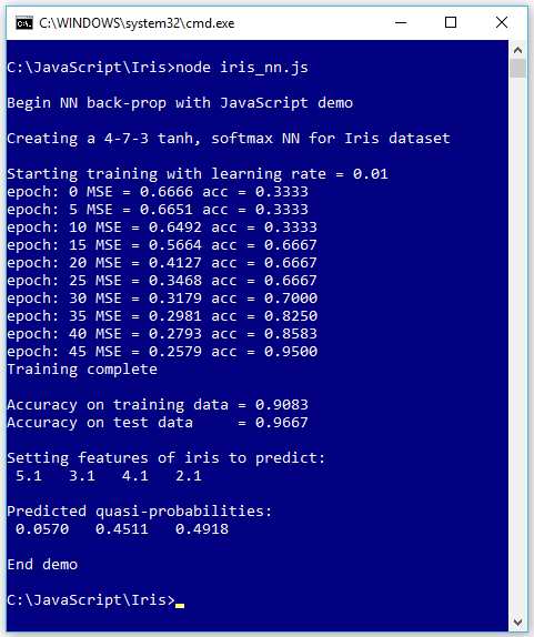
Figure 3-1: Neural Network Training on the Iris Data Set

The Iris data set has 150 data items. Each item represents an iris flower. There are four numeric predictor values (often called features in NN machine learning terminology) and three possible species to predict: setosa, versicolor, and virginica. The demo program creates a 4-7-3 neural network. There are four input nodes, one for each predictor value, and three output nodes, because there are three classes (discrete values to predict).

The neural network uses tanh activation on the hidden nodes and softmax output on the output nodes. Behind the scenes, the 150-item iris dataset had been split into two files: a 120-item (80% of the items) training data set to be used for determining the model weights and biases values, and a 30-item (the remaining 20%) test data set to be used to evaluate the quality of the trained network.

The demo program uses the back-propagation technique (also called stochastic gradient descent, SGD, even though the terms have somewhat different meanings) to train the network. Training is an iterative process. The demo program trains the network using 50 epochs. One epoch consists of processing every item in the training data set once.

During training, after each set of five epochs, the demo program displays the mean squared error associated with the current set of weights and biases, and the current prediction accuracy. As you can see in Figure 3-1, the error slowly decreases and the accuracy slowly increases, suggesting that training is working.

After training is completed, the demo computes and displays the prediction accuracy of the model on the 120-item training data (0.9083 = 109 out of 120 correct) and the 30-item test data (0.9667 = 29 out of 30 correct). The accuracy of the model on the test data set is a very rough estimate of the expected accuracy of the model on new, previously unseen data.

The demo program concludes by using the trained model to make a prediction. The demo sets up an iris flower with predictor values of (5.1, 3.1, 4.1, 2.1) and sends those values to the model. The model's output values are (0.0570, 0.4511, 0.4918). Because the third output value is the largest, the model predicts that the unknown flower is the third species (virginica).

Understanding the Iris data set

Fischer's Iris data set is one of the most well-known benchmark data sets in statistics and machine learning. The data set has 150 items. The raw data looks like this.

5.1, 3.5, 1.4, 0.2, setosa
7.0, 3.2, 4.7, 1.4, versicolor
6.3, 3.3, 6.0, 2.5, virginica
. . .

The raw data was prepared by one-hot encoding the class labels, but the feature values were not normalized as is usually done.

5.1, 3.5, 1.4, 0.2, 1, 0, 0
7.0, 3.2, 4.7, 1.4, 0, 1, 0
6.3, 3.3, 6.0, 2.5, 0, 0, 1
. . .

One-hot encoding is also known as 1-of-N encoding. The first class label gets a 1 in the first position, the second item gets a 1 in the second position, and so on. For example, if you are trying to predict the color of something, and there are four possible values (red, blue, green, yellow) then red = (1, 0, 0, 0), blue = (0, 1, 0, 0), green = (0, 0, 1, 0), and yellow = (0, 0, 0, 1).

The four predictor values are: sepal length, sepal width, petal length, and petal width. A sepal is a leaf-like structure.

After encoding, the full data set was split into a 120-item set for training and a 30-item test set to be used after training for model evaluation. The complete iris training and test data sets are presented in the appendix to this e-book.

Because the data has four dimensions, it's not possible to easily visualize it in a two-dimensional graph. But you can get a rough idea of the data from the partial graph in Figure 3-2.

As the graph shows, the Iris data set is quite simple. The setosa class can be easily distinguished from versicolor and virginica. Furthermore, the classes versicolor and virginica are nearly linearly separable. In spite of its simplicity, the Iris data set serves well as a classification example.

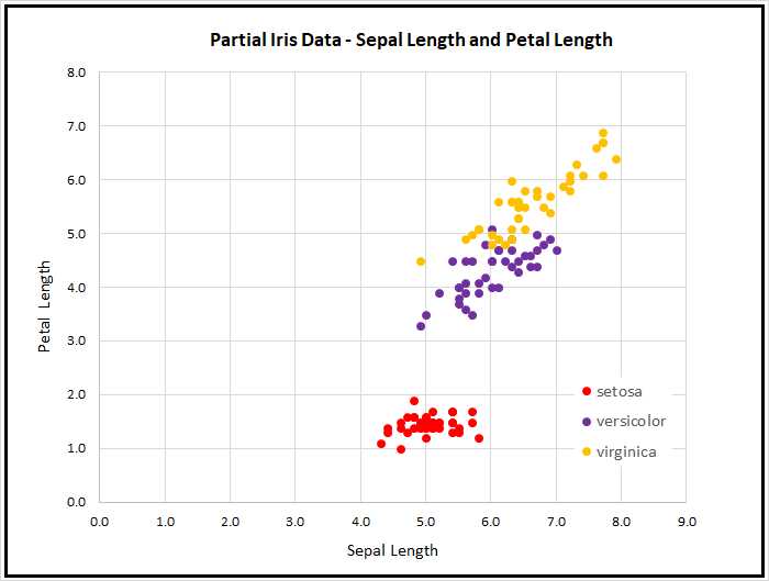
 Figure 3-2: The Iris data set

By the way, there are actually at least two different versions of Fisher's Iris data set that are in common use. The original data was collected in 1935 and published by Fisher in 1936. However, at some point in time, a couple of the original values for setosa items were incorrectly transcribed, and years later made their way onto the internet. This isn't serious because the data set is now used just for a teaching example rather than for serious research.

The Iris data set demo program utilities

The complete source code for the demo program is presented in Code Listings 3-1 and 3-2. The demo uses a file named Utilities_lib.js, which contains helper functions. The demo program is organized so that there is a top-level directory named JavaScript with subdirectories named Utilities and Iris. The Iris directory contains the Iris_nn.js demo program and a subdirectory named Data, which holds the files Iris_train.txt and Iris_test.txt.

The overall structure of the program is as follows.

// iris_nn.js
// ES6
let U = require("../Utilities/utilities_lib.js");

class NeuralNet
{
  . . . // define NN.
} 

function main
{
  // load training and test data into memory.
  let seed = 0;
  let nn = new NeuralNet(4, 7, 3, seed);  // create NN.
  // train the network.
  // evaluate the trained network.
  // use the trained network to make a prediction.
}

main();

It's possible to place all the utility functions in the same file as the core neural network functionality, but then the file becomes very large. When working with neural networks, you should not underestimate the importance of keeping your files organized.

Code Listing 3-1: File Utilities_lib.js Source Code

The Utilities_lib.js file contains 10 functions that work with vectors and matrices, one function named loadTxt() that reads data from a text file into memory, and one program-defined Erratic class to generate simple pseudo-random numbers.

The functions vecMake(), matMake(), vecShow(), and matShow() create and display JavaScript vectors and array-of-arrays style matrices.

The function softmax(vec) returns a vector of values scaled so that they sum to 1.0. For example, if vec = (3.0, 5.0, 2.0), then let sm = softmax(vec) returns a vector sm holding (0.1142, 0.8438, 0.0420). The function softmax() calls function vecMax(), which returns the largest value in a vector. For example, if a vector contained values (4.0, 3.0, 7.0, 5.0) then vecMax() returns 7.0.

The function hyperTan(x) returns the hyperbolic tangent of x. For example, hyperTan(-8.5) returns -1.0, hyperTan(9.5) returns 1.0, and hyperTan(1.1) returns 0.8005. The function logSig(x) returns the logistic sigmoid value of x.

The argmax(vec) function returns the index of its vector input parameter that has the largest value. For example, if a vector v contained values (4.0, 3.0, 7.0, 5.0), then argmax(v) returns 2.

The function arange(n) ("array-range") creates and returns a vector with values (0, 1, . . . n-1). For example, let v = arange(5) returns a vector v holding (0, 1, 2, 3, 4). The function is implemented.

function arange(n)
{
  let result = [];
  for (let i = 0; i < n; ++i) {
    result[i] = Math.trunc(i);
  }
  return result;
}

Because JavaScript does not have an integer data type, the values in the return vector are floating point values like (0.0, 1.0, 2.0, 3.0, 4.0), but it's conceptually convenient to think of the values as integers because they're used to represent array indices. Note that the call to the Math.trunc() function here has no significant effect, so it could have been omitted.

Reading data into memory

When training a neural network, the training and test data are usually stored as text files, so you need to read the data into memory. If your neural network code is client-side (in a browser), then you can use the XMLHttpRequest object to read from the server or the HTML5 FileReader object to read from the client machine. These techniques are outside the scope of this e-book.

If your neural network code is server-side and using Node.js, then you can use the Node.js File System library. The File System library is large (approximately 200 methods), and there are many ways to read a text file. The simplest approach when working with neural network data files is to use the readFileSync() function.

File utilities_lib.js implements a program-defined loadTxt() function. The implementation begins as follows.

let FS = require('fs');

function loadTxt(fn, delimit, usecols)
{
  let all = FS.readFileSync(fn, "utf8");
  all = all.trim();  // strip away last newline char.
. . .

The File System library is globally available and is accessed through the fs alias. The function loadTxt() has three parameters: fn, which is the name of the text file to read (including the path); delimit, which is a string defining the character that separates the numeric values on each line; and usecols, which is an array of indices indicating which columns to read. For example, suppose a text file named Dummy.txt is saved with UTF-8 encoding and has four lines.

1.3, 1.1, 1.9, 1.7
2.6, 2.8, 2.2, 2.4
3.2, 3.3, 3.0, 3.8

Then the statement let m = loadTxt(".\\dummy.txt", ",", [0,2,3]) would create a matrix m holding the following values.

1.30  1.90  1.70
2.60  2.20  2.40
3.20  3.00  3.80

The readFileSync() method reads the entire content of the text file into a variable as one giant string, including the newline characters at the end of each line. The File System library has a readFile() method that reads asynchronously, but the simpler readFileSync() works fine in most neural network scenarios.

The readFileSync() method assumes UTF-8 format by default, and also supports ascii, bae64, binary, hex, and latin1 encoding. The trim() function removes the trailing newline character, so variable all holds the following.

"1.3, 1.1, 1.9, 1,7 \n 2.6, 2.8, 2.2, 2.4 \n 3.2, 3.3, 3.0, 3.8 \n"

The implementation continues.

. . .
  let lines = all.split("\n");
  let rows = lines.length;
  let cols = usecols.length;
  let result = matMake(rows, cols, 0.0);

The call to split("\n") separates the one large string into separate strings.

lines[0] = "1.3, 1.1, 1.9, 1,7"
lines[1] = "2.6, 2.8, 2.2, 2.4"
lines[2] = "3.2, 3.3, 3.0, 3.8"

The implementation concludes.

. . .
   for (let i = 0; i < rows; ++i) {  // each line
    let tokens = lines[i].split(delimit);
    for (let j = 0; j < cols; ++j) {
      result[i][j] = parseFloat(tokens[usecols[j]]);
    }
  }

  return result;
}  

The call to split(",") peels off each numeric value, and then the call to parseFloat() converts the text representation of the current value into its numeric representation, which is then stored into the return-result matrix.

Reading data into memory for use by a neural network is simple in principle but is time-consuming and error-prone in practice. The demo code presented here can be used as a template for many neural network scenarios, but in situations where you need to write a different data reader, you should plan to spend several hours, or more, on development and testing.

Simple, pseudo-random numbers with an Erratic class

Neural networks use pseudo-random numbers when initializing weights and biases before training and to scramble the order in which training items are processed during training. One of the strange quirks of the JavaScript language is that the built-in Math.random() function does not have any way to set the random seed value, and therefore, there is no way to get reproducible results when using the function. Reproducible results are essential when working with neural networks.

Implementing a good pseudo-random number generator (where "good" means cryptographically secure and suitable for security-related usage) is extraordinarily difficult. Fortunately, neural networks don't require a sophisticated random number generator.

The Utilities_lib.js library contains a lightweight program-defined Erratic class. At a high level, in order to generate a pseudo-random value between 0.0 and 1.0, the idea is to compute the trigonometric sine function of the previous random value, and then peel off some of the trailing digits of the result.

The class is named Erratic rather than Random to emphasize the fact that the class is not a true pseudo-random number generator. The implementation looks like the following.

class Erratic
{
  constructor(seed) {
    this.seed = seed + 0.5;  // avoid 0
  }

  next() {
    // implementation here
  }

  nextInt(lo, hi) {
    // implementation here
  }
}

The class can be used as in the following.

let rnd = new Erratic(0);
let p = rnd.next();  // a pseudo-random value between [0.0, 1.0)
let ri = rnd.nextInt(0, 5);  // int-like value between [0, 5) = [0, 4]

The next() method returns a number in the range [0.0, 1.0), which means greater than or equal to 0.0 and strictly less than 1.0. The nextInt(lo, hi) method returns an integer-like number that is greater than or equal to lo and strictly less than hi. The nextInt() method is often used to select one cell of a vector. For example:

let v = vecMake(5, 0.0);  // a vector with 5 cells, each holding 0.0
let n = v.length;  // n is 5
let idx = rnd.nextInt(0, n);  // idx holds an index into v

The Erratic constructor() method accepts a seed value, which should be an integer-like number greater than or equal to 0. The internal this.seed value is set to the input seed plus 0.5 to avoid a seed of exactly 0, which would cause the next() method to generate a stream of only 0.0 values.

The next() method is implemented.

  next()
  {
    let x = Math.sin(this.seed) * 1000;
    let result = x - Math.floor(x);  // [0.0,1.0)
    this.seed = result;  // for next call
    return result;
  }

Initially, suppose a seed parameter of 0 was passed to the constructor() method. Then this.seed is 0.5 and x is computed as sin(0.5) * 1000 = 0.479425538604203 * 1000 =  479.425538604203. The Math.floor() function gives the integer part of its argument, and so x - Math.floor(x) = 0.425538604203. This value is returned by next(), and is also used as the new seed value the next time the next() method is called.

Notice that if the original seed value was exactly 0.0, then sin(0.0) = 0.0 and x - Math.floor(x) = 0.0, and therefore, the generator would emit an unending sequence of 0.0 values.

It’s very possible, but extremely unlikely, that after many thousands of calls to the next() method, a value of 0.0 could be generated. You could modify the next() method by adding a check.

  next()
  {
    let x = Math.sin(this.seed) * 1000;
    let result = x - Math.floor(x);  // [0.0,1.0)
    if (result == 0.0) {  // unlikely but possible
      throw("Zero error in call to Erratic.next()");
    }
    this.seed = result;  // for next call
    return result;
  }

There's usually a tradeoff between adding error-checking code and simplicity. The extent to which you'll want to add error checks will depend on your problem scenario.

It's convenient to have a method that returns an integer-like number, so the Erratic class defines a nextInt() method. The implementation is the following.

  nextInt(lo, hi)
  {
    let x = this.next();
    return Math.trunc((hi - lo) * x + lo);
  }

Suppose lo = 1 and hi = 7 (think the roll of a single dice). The internal call to this.next() will return a value in the range [0.0. 1.0). Multiplying that value by 7 - 1 = 6 will give a value in the range [0.0, 5.999999999]. Adding 1 will give a value in the range [1.0, 6.999999999]. Truncating will give a final value in the range [1, 6], or equivalently in the range [0, 7).

The Iris demo program code

The complete source code for the demo program is presented in Code Listing 3-2. The demo program begins by importing the functions in file Utilities_lib.js.

let U = require("../Utilities/utilities_lib.js");

The require() statement can handle either Windows-style file path strings with double backslash characters, or Linux-style strings with single forward slashes. Some programmers prefer to use the const keyword instead of let when importing a Node.js library using require().

Code Listing 3-2: File Iris_nn.js Source Code

The NeuralNet class constructor() accepts the number of input, hidden, and output nodes, and a seed value for an internal pseudo-random number generator.

class NeuralNet
{
  constructor(numInput, numHidden, numOutput, seed)
  {
    this.rnd = new U.Erratic(seed);
    this.ni = numInput;
    this.nh = numHidden;
    this.no = numOutput;
. . .

Notice that Erratic is defined in the Utilities_lib.js library file that's identified by U. Similarly, the calls to functions vecMake() and matMake() use the U identifier.

. . .
    this.iNodes = U.vecMake(this.ni, 0.0);
    this.hNodes = U.vecMake(this.nh, 0.0);
    this.oNodes = U.vecMake(this.no, 0.0);
    this.ihWeights = U.matMake(this.ni, this.nh, 0.0);
    this.hoWeights = U.matMake(this.nh, this.no, 0.0);
    this.hBiases = U.vecMake(this.nh, 0.0);
    this.oBiases = U.vecMake(this.no, 0.0);

    this.initWeights();

  } // constructor()

The last statement in the constructor() calls an initWeights() class method. This statement assigns small, random values to each of the network's weights and biases. Initialization of weights and biases is surprisingly subtle and important and will be explained shortly.

All of the program control logic is defined in a main() function. Program execution begins with the following.

function main()
{
  process.stdout.write("\033[0m");  // reset
  process.stdout.write("\x1b[1m" + "\x1b[37m");  // bright white
  console.log("\nBegin NN back-prop with JavaScript demo ");

  // 1. load data
  // data looks like: 5.1, 3.5, 1.4, 0.2, 1, 0, 0

  let trainX = U.loadTxt(".\\Data\\iris_train.txt", ",", [0,1,2,3]);
  let trainY = U.loadTxt(".\\Data\\iris_train.txt", ",", [4,5,6]);
  let testX = U.loadTxt(".\\Data\\iris_test.txt", ",", [0,1,2,3]);
  let testY = U.loadTxt(".\\Data\\iris_test.txt", ",", [4,5,6]);
. . .

When working with neural networks, it's common to load data into four matrices, as shown. It's good practice to add a comment in your code to explain the format of the data. The loadTxt() function does not support embedding comments in data files, but you can consider adding code to loadTxt() to allow comment lines.

The neural network is created like so.

  // 2. create network
  console.log("\nCreating a 4-7-3 tanh, softmax NN for Iris dataset");
  let seed = 0;
  let nn = new NeuralNet(4, 7, 3, seed);
. . .

Next, the network is trained with these statements.

  // 3. train network
  let lrnRate = 0.01;
  let maxEpochs = 50;
  console.log("\nStarting training with learning rate = 0.01 ");
  nn.train(trainX, trainY, lrnRate, maxEpochs);
  console.log("Training complete");
. . .

The train() method requires the known input values stored in the trainX matrix, and the known correct output values stored in the trainY matrix. The lrnRate (learning rate) variable controls how much each weight and bias value is changed on each training iteration. The maxEpochs variable sets a hard limit on the number of epochs, where an epoch consists of visiting and processing each training item one time.

Neural network training is extremely sensitive to the values used for the learning rate and the maximum number of training epochs. For example, a learning rate of 0.02 might work well, but a learning rate of 0.03 might cause the network to not learn at all.

The learning rate and maximum number of training epochs are called hyperparameters, which means you must specify their values and good values must be determined by trial and error. It's sometimes said that neural network expertise is part art and part science. The art component often refers to the idea that determining good hyperparameter values relies on experience.

During training, the train() method displays the values of the mean squared error and the classification accuracy, using the current values of the weights and biases. This is important because in nondemo problem scenarios, training failure is the rule rather than the exception. You want to identify situations where training is not working as quickly as possible.

After training, the trained model is evaluated.

  // 4. evaluate model
  let trainAcc = nn.accuracy(trainX, trainY);
  let testAcc = nn.accuracy(testX, testY);
  console.log("\nAccuracy on training data = " +
    trainAcc.toFixed(4).toString());
  console.log("Accuracy on test data     = " +
    testAcc.toFixed(4).toString());
. . .

The accuracy() method returns the classification accuracy of the model in decimal format, for example 0.9500, rather than in percentage format, like 95.00%. The demo program design has accuracy() as a class method, so it is called let acc = nn.accuracy(trainX, trainY). An alternative design is to implement accuracy() as a standalone function, in which case it would be called let acc = accuracy(nn, trainX, trainY).

Because the Iris data set problem is so simple, training is very quick. But realistic problems can require hours of training. The demo program does not save the trained model to file, but if training takes a long time, you'll usually want to save the values of the weights and biases to file.

The demo program concludes by making a prediction on a new, previously unseen iris flower.

  // 5. use trained model
  let unknown = [5.1, 3.1, 4.1, 2.1];  // set., set., ver., vir.
  let predicted = nn.eval(unknown);
  console.log("\nSetting features of iris to predict: ");
  U.vecShow(unknown, 1, 12);
  console.log("\nPredicted quasi-probabilities: ");
  U.vecShow(predicted, 4, 12);
. . .

The input values of (5.1, 3.1, 4.1, 2.1) are designed to be a challenge for the model. The first two predictor values (sepal length and width, 5.1, 3.1) are typical of those for the setosa species. The third predictor value (petal length, 4.1) is typical of versicolor, and the fourth predictor value (petal width, 2.1) is typical of virginica.

The eval() method returns a set of values (0.0570, 0.4511, 0.4918), and it's up to you to interpret the results. Because the third value is the largest, the model predicts the species of the unknown flower is the third species (virginica). If you wish, you can programmatically display the results.

  let species = ["setosa", "versicolor", "virginica"];
  let predIdx = U.argmax(predicted);
  let predSpecies = species[predIdx];
  console.log("Predicted species = " + predSpecies);

Even though the output values sum to 1.0 and can be loosely interpreted as probabilities, the values really aren't probabilities in the mathematical sense. However, the relative values do give you insights into how confident you can be of the prediction. In this case, because the pseudo-probabilities for versicolor and virginica are so close, you shouldn't have strong confidence in the prediction, compared to a result of something like (0.1000, 0.2000, 0.7000).

Weight and bias initialization

A neural network is very sensitive to the initial values of the weights and biases. The demo program uses the most basic form of initialization, which is to initialize all weights to small random values between -0.01 and +0.01, and to initialize all biases to 0.0 values. The class method initWeights() is defined.

  initWeights()
  {
    let lo = -0.01;
    let hi = 0.01;
    for (let i = 0; i < this.ni; ++i) {
      for (let j = 0; j < this.nh; ++j) {
        this.ihWeights[i][j] = (hi - lo) * this.rnd.next() + lo;
      }
    }

    for (let j = 0; j < this.nh; ++j) {
      for (let k = 0; k < this.no; ++k) {
        this.hoWeights[j][k] = (hi - lo) * this.rnd.next() + lo;
      }
    }
  }

Because the neural network architecture is 4-7-3, there are 4 * 7 = 28 input-to-hidden weights and 7 * 3 = 21 hidden-to-output weights. Each of these 49 weights is initialized to a random value between lo = -0.01 and hi = +0.01. All of the 7 + 3 = 10 biases in the network are left initialized to their original 0.0 values assigned in the constructor() method.

The limit values of (-0.01, +0.01) used for the weights are hyperparameters. Fixed weight initialization limit values usually work well with simple, single-hidden-layer networks, but often don't work well with deep neural networks. Researchers have devised several new advanced neural network weight initialization algorithms, including Glorot uniform, Glorot normal, He uniform, He normal, and LeCun normal.

Even though these advanced initialization algorithms were designed for use with deep neural networks, they often work very well with simple neural networks. The Glorot uniform algorithm can be implemented as in the following.

  initGlorotUniform()
  {
    let fanIn = this.ni;
    let fanOut = this.nh;

    let variance = 6.0 / (fanIn + fanOut);
    let lo = -variance; let hi = variance;

    for (let i = 0; i < this.ni; ++i) {
      for (let j = 0; j < this.nh; ++j) {
        this.ihWeights[i][j] = (hi - lo) * this.rnd.next() + lo;
      }
    }

    fanIn = this.nh;
    fanOut = this.no;

    variance = 6.0 / (fanIn + fanOut);
    lo = -variance; hi = variance;

    for (let j = 0; j < this.nh; ++j) {
      for (let k = 0; k < this.no; ++k) {
        this.hoWeights[j][k] = (hi - lo) * this.rnd.next() + lo;
      }
    }
  } // initGlorotUniform()

If you examine the code, you'll see that instead of initializing weights to small random values between arbitrary limits, the Glorot uniform algorithm determines the limit values based on the architecture of the network. In addition to usually working well, the Glorot uniform algorithm for initialization eliminates two hyperparameters that you have to deal with.

Error and accuracy

Classification accuracy and model prediction error are closely related. The key high-level takeaway idea is that you use error during training, and you use accuracy after training.

Suppose you have only three iris data items for training, and at some point during training, the current input and output values are the following.

input                target (correct)   computed
--------------------------------------------------------
5.0  3.5  1.5  0.5   1  0  0            0.70  0.20  0.10    
6.5  2.9  4.2  1.2   0  1  0            0.40  0.35  0.25
5.9  3.2  2.3  1.8   0  0  1            0.30  0.15  0.55

Accuracy is just the percentage of correct predictions. The input values and the known correct output values (often called the target values) are contained in the training data. The computed outputs are determined by the input values and the current values of the network weights and biases. For this data, the first and third items are correctly predicted, but the second item is incorrectly predicted. Therefore, the classification accuracy is 2 / 3 = 0.6667.

From a computational point of view, note that to determine if a set of computed output values gives a correct prediction, you can compare argmax(computed) and argmax(target) and check if the return indices are the same.

Accuracy is a relatively crude metric. You can imagine situations where the computed outputs are nearly perfect, for example, (0.9990, 0.0004, 0.0006) for the first item. And you can imagine situations where the computed outputs are just barely correct, for example, (0.3335, 0.3332, 0.3333) for the first item. But accuracy only counts correct-incorrect predictions.

In pseudo-code, the NeuralNet accuracy method is the following.

loop through each training data item
  computed = result of feeding item X vales to network
  target = item Y values
  if computed gives correct prediction
    increment correct counter
  else
    increment wrong counter
end-loop
return number correct / (number correct + number wrong)

The demo implementation.

  accuracy(dataX, dataY)
  {
    let nc = 0; let nw = 0;

    for (let i = 0; i < dataX.length; ++i) {  // each data item
      let X = dataX[i];
      let Y = dataY[i];  // target output like (0, 1, 0)

      let oupt = this.eval(X);  // computed output like (0.23, 0.66, 0.11)
      let computedIdx = U.argmax(oupt);
      let targetIdx = U.argmax(Y);

      if (computedIdx == targetIdx) {
        ++nc;
      }
      else {
        ++nw;
      }
    }

    return nc / (nc + nw);
  } // accuracy()

Compared to using a heavyweight neural network code library, such as TensorFlow or PyTorch, writing a lightweight implementation from scratch allows you to easily customize your code. For example, you might want to only count a prediction as correct if the computed output values are close to within some threshold value. Or you might want to insert console.log() messages to see exactly which input items are correctly predicted, and which are incorrectly predicted.

Mean squared error (MSE) is the average of the sum of the squared differences between the computed outputs and the correct target outputs. For example, the squared error terms for the three previous hypothetical data items are the following.

error(item 0) = (1 - 0.70)² + (0 - 0.20)² + (0 - 0.10)²  = 0.09 + 0.04 + 0.01 = 0.14
error(item 1) = (0 - 0.40)² + (1 - 0.35)² + (0 - 0.25)²  = 0.16 + 0.42 + 0.06 = 0.64
error(item 2) = (0 - 0.30)² + (0 - 0.15)² + (1 - 0.55)² = 0.09 + 0.02 + 0.20 = 0.31

Therefore, MSE = (0.14 + 0.64 + 0.31) / 3 = 1.09 / 3 = 0.36.

Notice that, mathematically, it doesn't matter if you compute (target - output)² or (output - target)². For example, (1 - 0.30)² = 0.70² = 0.49 and (0.30 - 1)² = -0.70² = 0.49. However, the order does matter when using the back-propagation technique, which relies on error. By far the more common of the two approaches is to use (target - output)², as the demo code does.

Additionally, instead of computing the error for each term and then summing those errors, you can just sum the squared differences between each component.

MSE = [ (1 - 0.70)² + (0 - 0.20)² + . . . + (1 - 0.55)² ] / 3 = (0.09 + 0.04 + . . . +0.20) / 3 = 0.36

In pseudo-code, the NeuralNet error method is this.

sumError = 0
loop through each training data item
  computed = result of feeding item X vales to network
  target = item Y values
  for each component in target, computed
    sumError += squared difference between component
  end-for
end-loop
return sumError / number training items

The demo implementation is this.

  meanSqErr(dataX, dataY)
  {
    let sumSE = 0.0;
    for (let i = 0; i < dataX.length; ++i) {  // each data item
      let X = dataX[i];
      let Y = dataY[i];  // target output like (0, 1, 0)

      let oupt = this.eval(X);  // computed like (0.23, 0.66, 0.11)

      for (let k = 0; k < this.no; ++k) {  // each component of target and computed
        let err = Y[k] - oupt[k]  // target - computed
        sumSE += err * err;
      }
    }

    return sumSE / dataX.length;
  }

Notice the parameter names for meanSqErr() are dataX and dataY rather than trainX and trainY or testX and testY to suggest that the function can be applied to either training data or test data. The statements let X = dataX[i] and let Y = dataY[i] retrieve a single row from the dataX and dataY matrices. The statements are just for clarity and the code could have used dataX[i] and dataY[i] directly.

Cross-entropy error

Cross-entropy error is a very important alternative to squared error. Cross-entropy error is also called log loss. The mathematical equation for cross-entropy error in the context of a neural network classifier is shown in Figure 3-3.

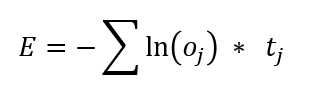
Figure 3-3: Cross-Entropy Error

In words, the cross-entropy error (CEE) for a single data item is the negative sum of the log of each computed output component times the target component. The idea is best explained by example.

Suppose you have only three iris data items for training a 4-7-3 neural network, and at some point during training, the current input and output values are (as in the previous section) this.

input                target (correct)   computed
--------------------------------------------------------
5.0  3.5  1.5  0.5   1  0  0            0.70  0.20  0.10    
6.5  2.9  4.2  1.2   0  1  0            0.40  0.35  0.25
5.9  3.2  2.3  1.8   0  0  1            0.30  0.15  0.55

The three cross-entropy error terms are the following.

error(item 0) = - [ ln(0.70) * 1  +  ln(0.20) * 0  + ln(0.10) * 0 ] = -ln(0.70) = 0.36
error(item 0) = - [ ln(0.40) * 0  +  ln(0.35) * 1  + ln(0.25) * 0 ] = -ln(0.35) = 1.05
error(item 0) = - [ ln(0.30) * 0  +  ln(0.15) * 0  + ln(0.55) * 1 ] = -ln(0.55) = 0.60

Therefore, the mean cross-entropy error = (0.36 + 1.05 + 0.60) / 3 = 2.01 / 3 = 0.67.

Cross-entropy error is quite subtle and isn't as easy to understand as squared error. Notice that when cross entropy is used for neural network classification, because there is only one 1 component in the target vector, only one term contributes to the result.

In practical terms, the key idea is that cross-entropy error is a value where smaller values mean less error between computed outputs and correct target outputs. Unlike squared error, which will always be a value between 0.0 and 1.0, cross-entropy error will always be greater than or equal to 0.0, but doesn't have an upper limit.

One possible implementation of mean cross-entropy error is this.

  meanCrossEntErr(dataX, dataY)
  {
    let sumCEE = 0.0;  // sum of the cross-entropy errors.
    for (let i = 0; i < dataX.length; ++i) {  // each data item.
      let X = dataX[i];
      let Y = dataY[i];  // target output like (0, 1, 0).

      let oupt = this.eval(X);  // computed like (0.23, 0.66, 0.11).

      let idx = U.argmax(Y);  // find location of the 1 in target.
      sumCEE += Math.log(oupt[idx]);
    }
   
    return -1 * sumCEE / dataX.length;
  }

Because the log(0) is negative infinity, this implementation could fail, for example, if target = (1, 0, 0) and computed = (0.0000, 0.7500, 0.2500). In practice, getting a computed output that has a 0.0000 component value associated with the target 1 component is extremely unlikely. But you could add an error check like this.

  . . .
  let idx = U.argmax(Y);  // find location of the 1 in target.
  if (oupt[idx] == 0.0) { // a really wrong output component.
    sumCEE += 100.0;  // an arbitrary large value, or could throw an Exception.
  }
  else {
    sumCEE += Math.log(oupt[idx]);
  }

As usual, adding error-checking code adds complexity. When writing your own lightweight neural network code, you can decide when and what type of error checking is needed.

Back-propagation training

Neural network training is the process of finding values for the network's weights and biases so that computed output values closely match the known, correct target values in the training data.

The back-propagation algorithm for neural network training is arguably one of the most important algorithms in the history of computer science. Back-propagation (often spelled as one word, backpropagation, due to a typo in a research paper decades ago that has been repeated ever since) is based on the general mathematical idea of stochastic gradient descent (SGD), and so the terms back-propagation and SGD are often used interchangeably.

Back-propagation is extraordinarily complex, but fortunately, a complete understanding of the theory is not necessary to implement the algorithm in practice. At a very high level, back-propagation training is as follows.

loop maxEpochs times
  for each training item
    get training item inputs X and correct target values Y
    compute output values using X  ("forward pass")

    (this is the "backward pass")
    compute the gradient of each hidden-output weight
    compute the gradient of each output node bias
    compute the gradient of each input-hidden weight
    compute the gradient of each hidden node bias

    use the gradients to adjust each weight and bias
  end-for
end-loop

Each neural network weight and bias has an associated value called a gradient. Technically, each value is a partial derivative of the weight with respect to the error function, but gradient is almost always used because it's much easier to say and write.

A gradient value has information about how the associated weight or bias value must change in order for computed output values to get closer to the target output values. This idea is illustrated in Figure 3-4. The graph represents one weight in a neural network. The possible values of the weight are shown on the horizontal axis at the bottom of the graph.

Each possible value of the weight will give a different error value. Therefore, the goal is to find the value of the weight that gives the smallest error. In the graph, you can see that the value of the weight that minimizes error is w = 5.0. Unfortunately, the error function is never completely known, so you can only take snapshots by sampling different values for w.

The gradient is the calculus derivative. A calculus derivative is the slope of the tangent line at some point. For example, if w = -5.0, you can see the error is about 7.0. The gradient at this point is -0.80 where the sign (negative in this case) indicates that the gradient runs from upper left to lower right. The magnitude of the gradient (0.80 in this case) indicates the steepness of the gradient.

If you examine the graph again, you can see than when w = -5.0 the gradient is negative, which means that to reduce error you must increase the value of w (towards 0).

The idea is also shown when w = 7.0. The gradient at that point is +2.15, and because the gradient is positive, to reduce the error you would decrease the value of w.

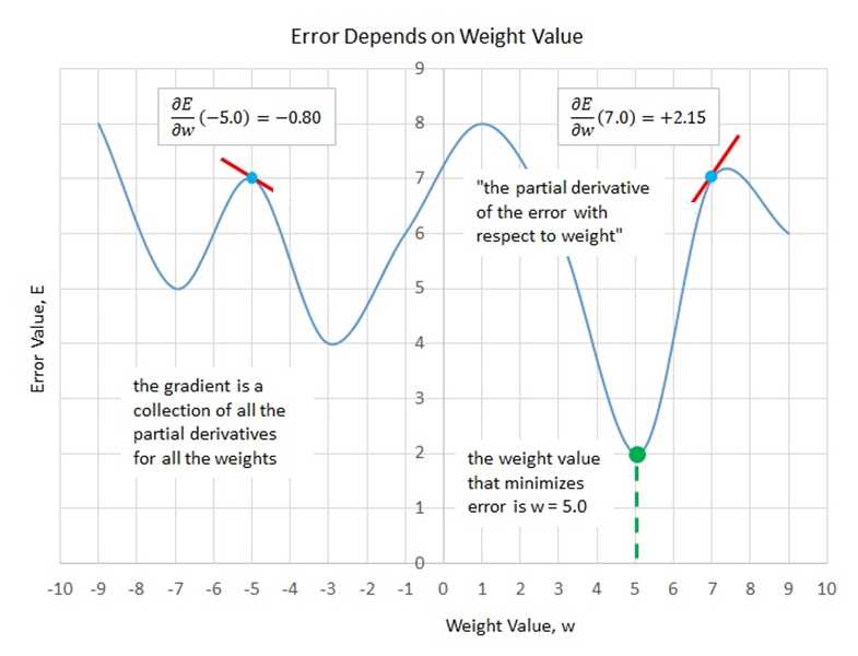
Figure 3-4: The Gradient of a Neural Network Weight

To summarize, if you can somehow compute the values of the gradients of each weight and bias, you can adjust the values of each weight and bias to reduce the error between computed output values and known correct output values. If the gradient is negative, increase the weight. If the gradient is positive, decrease the weight. Okay, but how can you compute gradients?

It turns out that calculating the gradients for the output node biases and the hidden-to-output weight is relatively simple, but calculating the gradients for the hidden node biases and the input-to-hidden weights is quite tricky.

Expressed as a math equation, the technique for updating the hidden-to-output weights and the output node biases is shown in Figure 3-5.

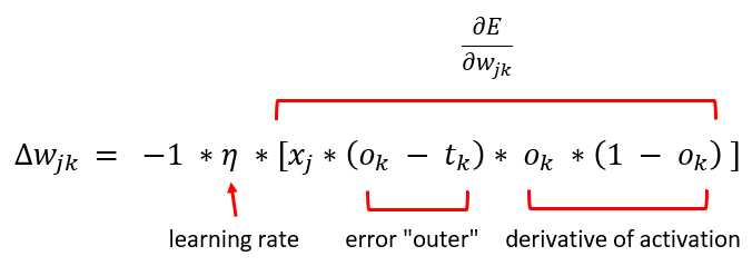
Figure 3-5: The Hidden-to-Output Weights Update Equation

The delta-w represents an increment of the weight from hidden node j to output node k that will decrease error. The -1 factor is an algebra consequence so that the delta value is added to the hidden-output weight rather than subtracted.

Greek letter eta (resembles a lower-case script "n") is the learning rate, which is a small value, typically something like 0.01 or 0.05. The x-j term is the value in the hidden node associated with the weight connecting hidden node j to output node k.

The (o - t) term ("output" minus "target") is part of a calculus derivative of the error function, in this case mean squared error. Notice that the back-propagation algorithm does not explicitly compute the error. Instead, the calculus derivative of the error function is used. If you use an error function other than mean squared error, the weight update equation changes.

The o * (1 - o) term is the calculus derivative of the output activation function, in this case the softmax function. If you use a different output activation function, the weight update equation changes. A technical exception to the fact that a change in activation function requires a change to the update calculation is that a neural network that uses logistic sigmoid output node activation has the same weight update equation as the equation assuming softmax. This happens because, mathematically, the softmax function and the logistic sigmoid function are very closely related.

Implementing back-propagation

Most of my software developer colleagues believe that the best way to understand back-propagation is to look at the code. The demo NeuralNet class implementation begins with the following.

  train(trainX, trainY, lrnRate, maxEpochs)
{
   let hoGrads = U.matMake(this.nh, this.no, 0.0);
   let obGrads = U.vecMake(this.no, 0.0);
   let ihGrads = U.matMake(this.ni, this.nh, 0.0);
   let hbGrads = U.vecMake(this.nh, 0.0);

   let oSignals = U.vecMake(this.no, 0.0);
   let hSignals = U.vecMake(this.nh, 0.0);
. . .

Because there is a gradient value for each weight and bias in the network, it makes sense to store those gradient values in matrices and vectors that have the same shape as the weights and the biases. For instance, hoGrads[3][0] holds the gradient for hoWeights[3][0], that is, the weight connecting hidden node [3] to output node [0].

The oSignals and hSignals vectors are scratch variables for computing the gradients, as you'll see shortly. The implementation continues as in the following.

  let n = trainX.length;  // 120
  let indices = U.arange(n);  // [0,1,..,119]
  let freq = Math.trunc(maxEpochs / 10);  // when to print error.
. . .

Variable n is the number of training items, 120 in this demo. The vector indices uses the arange() helper function to create a vector containing values (0, 1, . . n-1), which represent the indices of each training item. The idea here is that it's important in most cases to visit the training items in a different order every pass through the data set.

Variable freq (frequency) is a convenience to specify when to compute and print error and accuracy during training. In most nondemo situations, you don't want to compute and print these values for every training item because computing error and accuracy is computationally expensive, requiring iteration through the entire data set.

The 10 in the denominator means error and accuracy will be computed and displayed 10 times during training. For example, if maxEpochs is 350, then there will be information displayed 10 times (once every 35 epochs).

The main training loop begins with the following.

  for (let epoch = 0; epoch < maxEpochs; ++epoch) {
    this.shuffle(indices);
    for (let ii = 0; ii < n; ++ii) {  // each item
      let idx = indices[ii];

      let X = trainX[idx];
      let Y = trainY[idx];

      this.eval(X);  // output stored in this.oNodes.
. . .

Each epoch represents one complete pass through the training data. The demo code scrambles the order of the training items with the statement this.shuffle(indices). The class method shuffle() uses the Fisher-Yates algorithm to randomly rearrange the order of the index values in vector indices. The method is defined as follows.

  shuffle(v)
  {
    let n = v.length;

    for (let i = 0; i < n; ++i) {
      let r = this.rnd.nextInt(i, n);  // pick a random index.

      let tmp = v[r];  // exchange values.
      v[r] = v[i];
      v[i] = tmp;
    }
  }

The shuffle() method walks through its vector argument v and exchanges the values at randomly selected indices. The algorithm is surprisingly subtle. For example, incorrectly coding the statement this.rnd.nextInt(i, n) as this.rnd.nextInt(0, n) will generate strongly biased results. Also, notice that the loop condition i < n can be changed to i < n-1 because the last iteration exchanges the value in the last cell of vector v with itself.

The hidden-to-output weight gradients are computed by the following statements.

  // compute output node signals.
  for (let k = 0; k < this.no; ++k) {
    let derivative = (1 - this.oNodes[k]) * this.oNodes[k];  // assumes softmax.
    oSignals[k] = derivative * (this.oNodes[k] - Y[k]);  // E=(t-o)^2 do E'=(o-t)
  }

  // compute hidden-to-output weight gradients using output signals.
  for (let j = 0; j < this.nh; ++j) {
    for (let k = 0; k < this.no; ++k) {
      hoGrads[j][k] = oSignals[k] * this.hNodes[j];
    }
  }
. . .

The derivative term of the output signal depends on the output layer activation function. For softmax activation, the derivative is o * (1 - o), where o is the output node value. The computation for the oSignals vector values assumes that squared error is defined as (target - output)², which gives (output - target) because of the minus sign in the error term.

After the scratch output signals have been computed, the gradients are computed as the associated hidden node value times the output signal. None of these ideas is simple or obvious. From a developer's point of view, the idea to remember is that hidden-to-output weight gradients depend on the choice of error function and the choice of output layer activation function.

The gradients for the output node biases are computed like the following.

  // compute output node bias gradients using output signals.
  for (let k = 0; k < this.no; ++k) {
    obGrads[k] = oSignals[k] * 1.0;  // 1.0 dummy input can be dropped.
  }
. . .

The multiplication by the dummy 1.0 can be dropped because it doesn't affect the result. The idea here is that because a weight connects two nodes, you can think of a bias value as connecting one node with a constant 1.0 value. The use of the dummy 1.0 input value shows the symmetry between the computation of hidden-to-output weight gradients and the computation of the output node biases.

Next, the hidden node signals are computed using the output node signals and the calculus derivative of the hidden layer activation function, the hyperbolic tangent in this case.

  // compute hidden node signals.
  for (let j = 0; j < this.nh; ++j) {
    let sum = 0.0;
    for (let k = 0; k < this.no; ++k) {
      sum += oSignals[k] * this.hoWeights[j][k];
    }

    let derivative = (1 - this.hNodes[j]) * (1 + this.hNodes[j]);  // tanh
    hSignals[j] = derivative * sum;
  }
. . .

The ideas underlying this code are some of the deepest in all of machine learning. However, from a practical point of view, the only statement you'll ever need to change is the computation of the derivative term (if you decide to use a different hidden layer activation function). For example, if you use logistic sigmoid activation, because the calculus derivative of y = logsig(x) is y * (1 - y), the code changes to the following.

   let derivative = this.hNodes[j] * (1 - this.hNodes[j]);  // logistic sigmoid

Next, the gradients for the input-to-hidden weights and the gradients for the hidden node biases are computed.

  // compute input-to-hidden weight gradients using hidden signals.
  for (let i = 0; i < this.ni; ++i) {
    for (let j = 0; j < this.nh; ++j) {
      ihGrads[i][j] = hSignals[j] * this.iNodes[i];
    }
  }

  // compute hidden node bias gradients using hidden signals.
  for (let j = 0; j < this.nh; ++j) {
    hbGrads[j] = hSignals[j] * 1.0;  // 1.0 dummy input can be dropped.
  }
. . .

To summarize, the goal is to find a small delta value to add to each weight and bias so that computed outputs get closer to target output values (or equivalently, the error is reduced). To compute the delta values, you need to compute a gradient value for each weight and bias. The gradient values are composed of a signal and an input value (where the input value is a dummy 1.0 for biases).

After the gradients have been computed, the next step is to compute the delta values and then use them to modify the weights and biases. When computing the gradients, you must work backward from output to hidden to input (which is why back-propagation is named as it is). But when updating the weights and biases, you can work in any order. The demo code works from input to hidden to output to emphasize that the order of weights and biases updates can be different from the order of gradient computations.

The train() method continues by updating the input-to-hidden weights.

  // update input-to-hidden weights
  for (let i = 0; i < this.ni; ++i) {
    for (let j = 0; j < this.nh; ++j) {
      let delta = -1.0 * lrnRate * ihGrads[i][j];
      this.ihWeights[i][j] += delta;
    }
  }
. . .

If you compare this code with the weight update equation in Figure 3-5, you will see a one-to-one correspondence between the code and the math. Recall that the purpose of the -1 term is just so that the weight value is updated by adding using the += operator. Instead, you could write the following equivalent code.

  let delta = lrnRate * ihGrads[i][j];
  this.ihWeights[i][j] -= delta;

In other words, instead of multiplying by -1 to get a negative value and then adding, you can just subtract. Even though this alternative approach is a tiny bit more efficient (saving a multiplication by -1 operation), it's rarely used. Next, the hidden node biases are updated using their associated gradients.

  // update hidden node biases.
  for (let j = 0; j < this.nh; ++j) {
    let delta = -1.0 * lrnRate * hbGrads[j];
    this.hBiases[j] += delta;
  }
. . .

The pattern to update biases is exactly the same as the pattern used to update weights. Next, the hidden-to-output weights and the output node biases are updated.

    // update hidden-to-output weights.
    for (let j = 0; j < this.nh; ++j) {
      for (let k = 0; k < this.no; ++k) {
        let delta = -1.0 * lrnRate * hoGrads[j][k];
        this.hoWeights[j][k] += delta;
      }
    }

    // update output node biases.
    for (let k = 0; k < this.no; ++k) {
      let delta = -1.0 * lrnRate * obGrads[k];
      this.oBiases[k] += delta;
    }
  } // each item
. . .

At this point, every data item in the training data set has been read and processed once, and each item generates an update for each weight and bias. In the demo, there are 120 training items, and the neural network architecture is 4-7-3, so there are (4 * 7) + 7 + (7 * 3) + 3 = 59 weights and biases. Therefore, one pass through the training data set (called an epoch) produces 120 * 59 = 7,080 update operations in one epoch. The demo program sets the number of epochs to 50, so the entire program generates 7080 * 50 = 354,000 update operations.

The train() method concludes by checking to see if it's time to show a progress message.

. . .
      if (epoch % freq == 0) {
        let mse = this.meanSqErr(trainX, trainY).toFixed(4);
        let acc = this.accuracy(trainX, trainY).toFixed(4);

        let s1 = "epoch: " + epoch.toString();
        let s2 = " MSE = " + mse.toString();
        let s3 = " acc = " + acc.toString();

        console.log(s1 + s2 + s3);
      }
    } // epoch
  } // train()

Checking for progress messages is placed at the end of the main processing loop. You could check at the top of the main loop.

. . .
  for (let epoch = 0; epoch < maxEpochs; ++epoch) {  // each epoch.
    this.shuffle(indices);                           // scramble order of items.
    for (let ii = 0; ii < n; ++ii) {                 // each training item.
    if (epoch % freq == 0) {                         // it's time to show progress.
      let mse = this.meanSqErr(trainX, trainY).toFixed(4);
. . .

Using this approach would display the mean squared error and classification accuracy immediately (at epoch = 0), which is useful to get baseline values. The disadvantage is that during all other epochs, you see error and accuracy of the model before weights and biases are updated, not after the updates.

Back-propagation using cross-entropy error

In spite of decades of research on neural networks, many fundamental questions remain unanswered. One such question is, "For neural multiclass classification, should you use mean squared error or cross-entropy error?" In my opinion, there are no definitive research results that answer this question. For some problems, mean squared error seems to work better, but for other problems, mean cross-entropy error appears to work better.

For a multiclass classification problem, to use mean cross-entropy error instead of mean squared error, you only need to make one small (but truly surprising) change to the demo code. When using mean squared error, the statements that compute the output node signals are the following.

  // compute output node signals (assuming mean squared error).
  for (let k = 0; k < this.no; ++k) {
    let derivative = (1 - this.oNodes[k]) * this.oNodes[k];  // assumes softmax.
    oSignals[k] = derivative * (this.oNodes[k] - Y[k]);  // E=(t-o)^2 do E'=(o-t)
  }

Because of some algebra cancellations, when using mean cross-entropy error, the computation of the output node signals becomes the following.

  // compute output node signals (assuming mean cross-entropy error).
  for (let k = 0; k < this.no; ++k) {
    // assumes softmax.
    oSignals[k] = this.oNodes[k] - Y[k];  // E=-Sum(ln(o)*t)
  }

The derivative term essentially goes away, leaving just the (output - target) term. This is one of the most surprising results in all of neural machine learning.

The demo program displays error and accuracy progress messages during training. If you use mean cross-entropy error instead of mean squared error, it makes sense to display mean cross-entropy error rather than mean squared error. But because mean squared error is slightly easier to interpret than cross-entropy error, you might want to display both error metrics.

  if (epoch % freq == 0) {  // time to display progress.
    let mse = this.meanSqErr(trainX, trainY).toFixed(4);
    let mcee = this.meanCrossEntErr(trainX, trainY).toFixed(4);
    let acc = this.accuracy(trainX, trainY).toFixed(4);

    let s1 = "epoch: " + epoch.toString();
    let s2 = " MSE = " + mse.toString();
    let s3 = " MCEE = " + mcee.toString();
    let s4 = " acc = " + acc.toString();

    console.log(s1 + s2 + s3 + s4);
  }

Until the year 2012 or so, the use of mean squared error was more common than the use of mean cross-entropy error. However, cross-entropy error is now far more common. The graph in Figure 3-6 shows an example of squared error and cross-entropy error applied to the same problem.

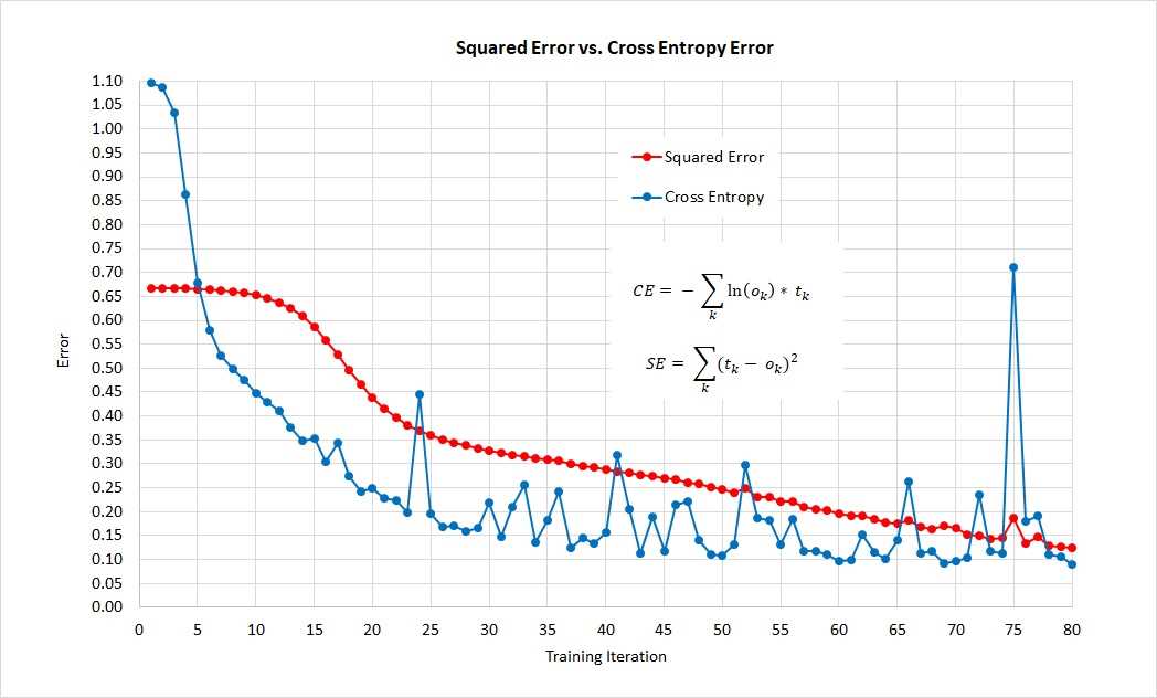
Figure 3-6: Comparison of Squared Error and Cross-Entropy Error on Same Problem

The graph shows that, for this one problem, cross-entropy error gives a good neural network model more quickly than squared error, but that cross entropy is more volatile than squared error.

In practice, if you use enough training iterations, for most multiclass classification problems mean squared error and mean cross-entropy error produce similar neural network models in terms of prediction accuracy. However, because cross-entropy error is used much more often than squared error, you should use cross-entropy error if you are collaborating with others. And note that for regression problems, where the goal is to predict a single numeric value, cross-entropy error is not an option.

Although the terms back-propagation and stochastic gradient descent are often used interchangeably, they're different. Technically, the back-propagation algorithm computes calculus gradients, and stochastic gradient descent uses the gradients to reduce error.

Stochastic gradient descent often works quite well for neural networks with a single hidden layer, but often fails for deep neural networks. Between 2014 and 2017, remarkable progress was made in devising powerful new learning algorithms for deep neural networks. Most of these algorithms use a different learning rate for each weight and bias, and adaptively change the learning rates during training.

Advanced algorithms supported by most deep neural network code libraries such as TensorFlow and PyTorch include Adagrad (adaptive gradient), Adadelta (improved variation of Adagrad), RMSProp (adaptive gradient plus resilient back-prop), Adam ("adaptive moment estimation," similar to RMSProp with momentum), and AdaMax (a variation of Adam).

All of these learning algorithms are based on calculus gradients. There are exotic learning algorithms that don't rely on gradients. For example, evolutionary optimization is similar to genetic algorithms that loosely mimic the behavior of biological chromosomes. And particle swarm optimization loosely mimics the behavior of swarming organisms. These bio-inspired techniques have great promise, but are currently not practical because they require truly enormous computational power.

Questions

1. Suppose that at some point during training, a neural network's current input and output values are the following.

input                   target        computed
--------------------------------------------------------
4.8  3.9  1.1  0.8      1  0  0       0.80  0.10  0.10    
6.7  2.6  4.6  1.3      0  1  0       0.15  0.60  0.25
5.6  3.1  2.2  1.7      0  0  1       0.20  0.50  0.30

1. What is the classification accuracy of the network?
2. What is the mean squared error of the network?
3. What is the mean cross-entropy error of the network?