Overfitting

---

One of the big challenges when working with neural networks is a phenomenon called overfitting. A trained model is overfitted if it predicts well on the training data but predicts poorly on test data and new, previously unseen data. There are many techniques to reduce the likelihood of model overfitting, including dropout, train-validate-test, and regularization.

The screenshot in Figure 4-1 shows a demo of neural network overfitting. The goal of the program is to predict the political leaning of a person (conservative, moderate, or liberal) based on sex (male or female), age, geographical region (eastern, western, or central), and annual income.

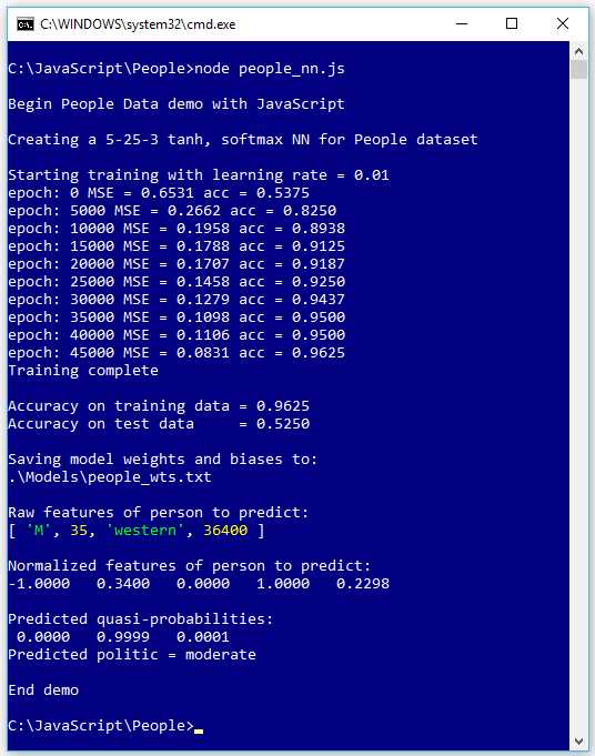
Figure 4-1: An Example of Neural Network Model Overfitting

The data is completely artificial and was generated programmatically. The raw data has 240 items that look like the following.

M 32 eastern 59200.00 | moderate
F 33 central 38400.00 | moderate
M 35 central 30800.00 | liberal
M 26 western 53800.00 | conservative
. . .

The first column is the person's sex, represented by M or F. The second column is the person's age. The third column is the geo-region (eastern, western, or central) where the person lives. The fifth column is an arbitrary pipe character for readability. The sixth column is the political leaning to predict (conservative, moderate, or liberal).

The 240-item raw data was split into a 160-item data set for training and a 40-item data set for testing. After splitting, the two data sets were normalized and encoded for use by a neural network (the remaining 40 items are used later).

The demo created a 5-25-3 neural network. The raw data has four predictor variables, but when normalized and encoded, there are five predictor values. There are three output nodes because there are three classes to predict. The number of hidden nodes (25) is a hyperparameter and must be determined by trial and error.

The demo program trains the network for 50,000 epochs using back-propagation with the online training technique. After training, the model's classification accuracy is an impressive 96.25% correct (154 out of 160), but a rather unimpressive 52.50% accuracy (21 out of 40) on the test data. The difference in prediction accuracy on the training and test datasets suggest that the model has been overfitted.

After the model evaluation metrics have been displayed, the demo saves the model's weights and biases to a text file so that they can be retrieved later. For all but the quickest training, you'll want to save your model weights and biases so you don't have to retrain a good model.

The demo concludes by making a prediction for a new, previously unseen person with raw predictor values of sex = male, age = 35, region = "western", and income = $36,400.00. These values are normalized and encoded to sex = -1, age = 0.3400, region = (0, 1), and income = 0.2298. The prediction probabilities are (0.0000, 0.9999, 0.0001), and because the second value is largest, the prediction is that the person is a political moderate. The extreme values of the predicted probabilities also suggest the model may be overfitted.

The graph in Figure 4-2 illustrates the basic concepts of overfitting. In the figure, there are two predictor variables, X1 and X2. There are two possible values to predict, indicated by the red (class = 0) and blue (class = 1) dots. You can imagine this corresponds to the problem of predicting if a person is male (0) or female (1), based on normalized age (X1) and normalized income (X2). For example, the left-most data point at (X1 = 1, X2 = 4) is colored blue (female).

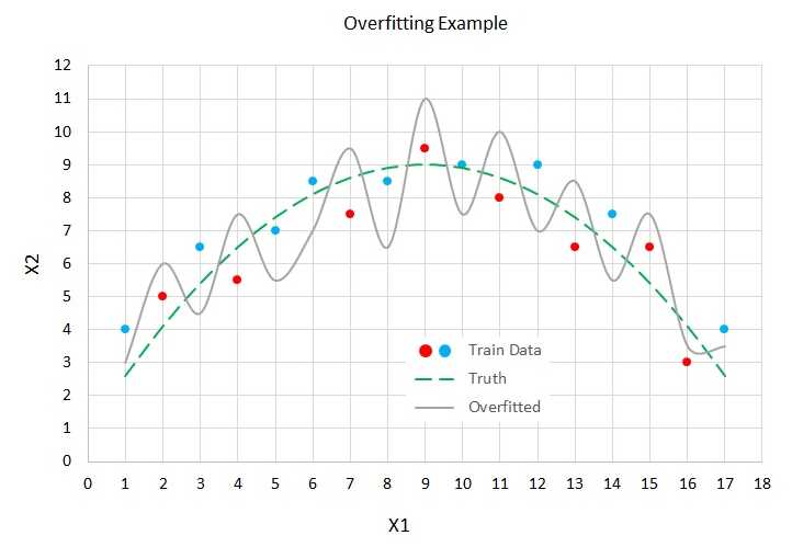
Figure 4-2: Model Overfitting

The dashed green line represents the true (but unknown) decision boundary between the two classes. Notice that data items that are above the green line are mostly blue (seven of ten), and that data items below the green line are mostly red (five of seven). The five misclassifications in the training data are due to the randomness inherent in all real-life data.

A good neural network model would find the true decision boundary represented by the green line. However, if you train a neural network model long enough, it will essentially get too good and generate a model indicated by the spiky, solid gray line.

The gray line makes perfect predictions on the test data. All the blue dots are above the gray line and all the red dots are below the gray line.

But when the overfitted model is presented with new, previously unseen data, there's a good chance the model will make an incorrect prediction. For example, a new data item at (X1 = 4, X2 = 7) is above the truth boundary, and so should be classified as blue. But because the data item is below the gray line overfitted boundary, it will be incorrectly classified as red.

Data normalization

Preparing data for use by a neural network is often tedious and time-consuming. In most scenarios there are three distinct data preparation tasks: cleaning, normalizing numeric data, and encoding non-numeric data.

Cleaning data usually means dealing with missing values and extreme or anomalous values. For data items that have one or more missing predictor values, in all but rare cases the best approach (in my opinion) is to delete those data items. Alternatives such as supplying an average value of some sort are sometimes used in classical statistics scenarios, but such techniques rarely work well with neural networks.

In almost all neural network scenarios, you should normalize numeric predictor values so that the values are scaled to roughly the same magnitude. Note that the Iris data set in Chapter 3 is an exception because the data is so simple and is already scaled to values between 0.1 and 7.9 (this is a major reason why the Iris data set is used so often for neural network examples).

The three most common forms of data normalization are min-max normalization, z-score normalization, and constant factor normalization. All three techniques are best explained by example.

Suppose you have a tiny set of training data with just three items.

25   68000.00   male     moderate
41   73000.00   male     conservative
36   54000.00   female   liberal

The goal is to predict political leaning from age, annual income, and sex. Without normalization, the large annual income values would overwhelm the small age values.

To apply min-max normalization to a numeric predictor, you find the minimum and maximum value in its column, then compute (x - min) / (max - min).

For the age variable, min = 25 and max = 41, and so the normalized age values are the following.

(25 - min) / (max - min) = (25 - 25) / (41 - 25) = 0.0000
(41 - min) / (max - min) = (41 - 25) / (41 - 25) = 1.0000
(36 - min) / (max - min) = (36 - 25) / (41 - 25) = 0.6875

The annual income values could be normalized in the same way.

(68000 - min) / (max - min) = (68000 - 54000) / (73000 - 54000) = 0.7368
(73000 - min) / (max - min) = (73000 - 54000) / (73000 - 54000) = 1.0000
(54000 - min) / (max - min) = (54000 - 54000) / (73000 - 54000) = 0.0000

After min-max normalizing a numeric predictor variable, all values will be scaled between 0.0 and 1.0.

To apply z-score normalization, you find the mean and standard deviation for each numeric column, then compute (x - mean) / sd.

For the age variable, mean = 34.00 and sd = 6.68, and so the normalized values are the following.

(25 - mean) / sd = (25 - 34.00) / 6.68 = -1.3473
(41 - mean) / sd = (41 - 34.00) / 6.68 = 1.0479
(36 - mean) / sd = (36 - 34.00) / 6.68 = 0.2994

After z-score normalizing a predictor variable, the values will usually be between -5.0 and +5.0. Normalized values less than -5.0 or greater than 5.0 are extreme in the sense that they're much different from the average value.

To apply constant factor normalization, you divide or multiply all values by a constant. For example, for the age values, you could divide each value by 100.

25 / 100 = 0.25
41 / 100 = 0.41
36 / 100 = 0.36

In general, there is no one best normalization technique. In practice, the type of normalization technique used usually doesn't have a huge effect on the prediction accuracy of the trained network. It is possible to use different normalization techniques on different predictors in your training data. For example, you could normalize age values using min-max normalization and normalize annual income values using z-score normalization.

After normalizing your training data, you must use the same normalizing parameters on the test data. For example, suppose you have a set of training data where one of the predictors is a person's height in inches. If you use min-max normalization on the training data where min = 58.0 and max = 77.0, then when you normalize the test data, you do not calculate a new min and max value. You use the min = 58.0 and max = 77.0 on the test data, regardless of the actual min and max values in the test data.

In short, the steps are:

1. Split all data into a training and a test set.
2. Normalize the training data.
3. Normalize the test data using the normalization parameters from the training data.

Data encoding

A neural network works directly only with numeric values, so predictor variables that are non-numeric (sometimes called categorical) must be converted to numbers. For categorical predictor variables that can take one of three or more values, the two most common encoding techniques are 1-of-(N-1) encoding and one-hot encoding (sometimes called 1-of-N encoding). For categorical predictor variables that can take one of just two possible values (binary predictors), the three most common encoding techniques are one-hot encoding, -1 +1 encoding, and 0-1 encoding.

Before explaining these techniques, let me say that my recommendations are to use 1-of-(N-1) encoding for predictors that can be from three to nine possible values, use one-hot encoding for predictors that can be 10 or more possible values, and use -1 +1 encoding for binary predictors that can be one of two possible values.

Suppose you have a categorical predictor variable, color, that can be one of four possible values: red, blue, green, yellow. If you use one-hot / 1-of-N encoding, then red = (1, 0, 0, 0), blue = (0, 1, 0, 0), green = (0, 0, 1, 0), and yellow = (0, 0, 0, 1).

If you use 1-of-(N-1) encoding, then red = (1, 0, 0), blue = (0, 1, 0), green = (0, 0, 1), and yellow = (-1, -1, -1). The 1-of-(N-1) encoding technique is sometimes called effect coding or contrast coding, but there is quite a bit of inconsistency with the terminology.

Suppose you have a binary predictor variable, sex, that can be either male or female. If you use one-hot encoding, then male = (1, 0) and female = (0, 1). If you use -1 +1 encoding, then male = -1 and female = +1. If you use 0-1 encoding, then male = 0 and female = 1.

If you have a classification problem, then you must encode the values of the variable to predict (the dependent variable), too. For dependent variables that can be one of three or more values (such as political leaning of conservative, moderate, or liberal), then you should always use one-hot / 1-of-N encoding: conservative = (1, 0, 0), moderate = (0, 1, 0), liberal = (0, 0, 1).

For binary classification problems (such as predicting a person's sex of male or female), by far the most common approach is to use 0-1 encoding: male = 0, female = 1. However, you can also use one-hot / 1-of-N encoding: male = (1, 0), female = (0, 1). Encoding a binary dependent variable for a neural network is surprisingly subtle, and is explained in Chapter 6, Binary Classification.

Understanding the People Dataset

The People Dataset consists of 240 tab-delimited items. The data was split into a training set of 160 items and a test set of 40 items. The training set raw data looks like the following.

M 32 eastern 59200.00 | moderate
F 33 central 38400.00 | moderate
M 35 central 30800.00 | liberal
M 26 western 53800.00 | conservative
. . .

The training set was normalized using min-max normalization on both the age (min = 18, max = 68) and the annual income (min = 20,500.00, max = 89,700.00) predictor variables.

The sex predictor variable was encoded as M = -1 and F = +1. The region predictor variable was 1-of-(N-1) encoded as eastern = (1, 0), western = (0, 1), central = (-1, -1). The dependent variable to predict, political leaning, was one-hot encoded as conservative = (1, 0, 0), moderate = (0, 1, 0), liberal = (0, 0, 1). The normalized and encoded training data looks like the following.

-1  0.28   1  0  0.5592   0 1 0
1  0.30  -1 -1  0.2587   0 1 0
-1  0.34  -1 -1  0.1488   0 0 1
-1  0.16   0  1  0.4812   1 0 0
. . .

The 40-item test data was min-max normalized using the training data age parameters (min = 18, max = 68) and annual income parameters (min = 20,500, max = 89,700), and was encoded. The test data looks like the following.

 1  1.00  -1 -1  0.4581   1 0 0
1  0.68   1  0  0.9682   1 0 0
-1  0.70   1  0  0.1705   0 1 0
. . .

Even this tiny data set took quite some time to prepare. In practice, it's rarely possible to experiment with different normalization and encoding schemes, so you must decide beforehand which techniques to use.

The normalized and encoded data used by the demo programs are in the appendix to this e-book, and on GitHub.

The People Dataset demo program

The complete demo program shown running in Figure 4-1 is presented in Code Listing 4-1. The demo assumes there is a top-level directory named JavaScript that contains subdirectories named Utilities and People. The Utilities directory contains the Utilities_lib.js library file. The People directory contains the demo program People_nn.js file and subdirectories named Data and Models. The Data directory contains files People_train.txt and People_test.txt. The Models directory is used to store trained model weights and biases values.

Code Listing 4-1: The People Data Demo Program

All of the control logic is contained in a top-level main() function. Program execution begins by loading the training and test data into memory.

  // 1. load data
  // raw data looks like:   M   32   western  38400.00    |  moderate
  // norm data looks like: -1  0.28    0 1    0.2587          0 1 0
  let trainX = U.loadTxt(".\\Data\\people_train.txt", "\t", [0,1,2,3,4]);
  let trainY = U.loadTxt(".\\Data\\people_train.txt", "\t", [5,6,7]);
  let testX = U.loadTxt(".\\Data\\people_test.txt", "\t", [0,1,2,3,4]);
  let testY = U.loadTxt(".\\Data\\people_test.txt", "\t", [5,6,7]);
. . .

The loadTxt() function is contained in the Utilities_lib.js file, which is located in the Utilities directory. Notice that the data files are tab-delimited. Next, a neural network is created.

  // 2. create network
  console.log("\nCreating a 5-25-3 tanh, softmax NN for People dataset");
  let seed = 0;
  let nn = new NeuralNet(5, 25, 3, seed);
. . .

The raw data has four predictor variables (sex, age, region, and income), but there are five predictor values after normalization because region has been 1-of-(N-1) encoded. The number of hidden nodes, 25, is a hyperparameter that must be determined by trial and error. In general, more hidden nodes can produce a more accurate model at the expense of an increased risk of model overfitting. The seed value is for random initialization of weights and random order processing of training items. Next, the network is trained.

  // 3. train network
  let lrnRate = 0.01;
  let maxEpochs = 50000;
  console.log("\nStarting training with learning rate = 0.01 ");
  nn.train(trainX, trainY, lrnRate, maxEpochs);
  console.log("Training complete");
. . .

The large number of training iterations (50,000) could lead to overfitting. Next, the trained mode is evaluated.

  // 4. evaluate model
  let trainAcc = nn.accuracy(trainX, trainY);
  let testAcc = nn.accuracy(testX, testY);

  console.log("\nAccuracy on training data = " +
    trainAcc.toFixed(4).toString());

  console.log("Accuracy on test data     = " +
    testAcc.toFixed(4).toString());
. . .

The end goal of a neural network classifier is prediction accuracy, so it makes sense to compute accuracy after training. In many cases you'll also want to compute and display the trained model's error (either mean squared error or mean cross-entropy error, or both), for example, with code similar to the following.

let trainError = nn.MeanSqErr(trainX, trainY);
console.log(trainError.toFixed(4).toString());

Error is a useful metric for comparing different trained models because error is a more granular metric than accuracy. Next, the trained model's weights and biases are saved to a text file.

  // 5. save model
  let fn = ".\\Models\\people_wts.txt";
  console.log("\nSaving model weights and biases to: ");
  console.log(fn);
  nn.saveWeights(fn);
. . .

The demo program concludes by making a prediction for a new, previously unseen person.

  // 6. use trained model
  let unknownRaw = ["M", 35, "western", 36400.00];
  let unknownNorm = [-1, 0.34, 0, 1, 0.2298];

  let predicted = nn.eval(unknownNorm);

  console.log("\nRaw features of person to predict: ");
  console.log(unknownRaw);

  console.log("\nNormalized features of person to predict: ");
  U.vecShow(unknownNorm, 4, 12);

  console.log("\nPredicted quasi-probabilities: ");
  U.vecShow(predicted, 4, 12);
. . .

The demo program normalizes and encodes the new person item offline. An alternative that is useful when making many predictions is to write a problem-specific function to normalize and encode. For example, using such a function might look like the following.

let unknownRaw = ["F", 27, "eastern", 42500.00];
let unkNorm = normAndEncode(unknownRaw);
let predicted = nn.eval(unkNorm);

Note that a program-defined function to normalize and encode raw data needs to know the normalization parameters, such as min and max if min-max normalization is used.

The demo program wraps up by displaying the predicted political leaning in user-friendly form.

  let politics = ["conservative", "moderate", "liberal"];
  let predIdx = U.argmax(predicted);
  let predPolitic = politics[predIdx];
  console.log("Predicted politic = " + predPolitic);

The pattern used in the demo is: load data, create neural network, train network, evaluate network, save weights and biases, and use model. This pattern, or one very close to it, is a very common pattern when working with neural networks.

Saving and loading model weights

The NeuralNet class method saveWeights() is defined as the following.

  saveWeights(fn)
  {
    let wts = this.getWeights();
    let n = wts.length;
    let s = "";

    for (let i = 0; i < n-1; ++i) { // all except last value.
      s += wts[i].toString() + ",";
    }
    s += wts[n-1];  // last value, no trailing comma.

    FS.writeFileSync(fn, s);
  }

The statement let wts = this.getWeights() returns a vector named wts with the weights and biases serialized as the input-to-hidden weights, followed by the hidden node biases, followed by the hidden-to-output weights, followed by the output node biases. Because the demo network has a 5-25-3 architecture, there are a total of (5 * 25) + 25 + (25 * 3) + 3 = 228 weights and biases. The weights and biases are serialized to a single, comma-separated string (without a trailing comma), which is written to a text file.

There are many alternative designs you can use. For example, you might want to write an architecture such as 5,25,3 and then follow with the weights and biases, or you might want to write the weights using JSON or XML format, and so on.

Almost all widely used deep neural network libraries, such as TensorFlow, Keras, and PyTorch, save models in a proprietary binary format. However, many of these libraries have added support for the ONNX (open neural network exchange) standard.

The counterpart to saveWeights() is a method loadWeights() that loads saved weights from file into a neural network. A loadWeights() method can be defined as the following.

  loadWeights(fn)
  {
    let n = (this.ni * this.nh) + this.nh + (this.nh * this.no) + this.no;
    let wts = U.vecMake(n, 0.0);

    let all = FS.readFileSync(fn, "utf8");
    let strVals = all.split(",");
    let nn = strVals.length;

    if (n != nn) {
      throw("Size error in NeuralNet.loadWeights()");
    }

    for (let i = 0; i < n; ++i) {
      wts[i] = parseFloat(strVals[i]);
    }
    this.setWeights(wts);
  }

The method sets up a numeric vector to hold the serialized weights and biases, then reads all those values from file into a single large string. The string is split on the comma characters, and then the individual values are converted to numeric form and placed into the vector. The vector is then passed to the class setWeights() method, which places the values into the neural network.

Method loadWeights() can be called along the lines of the following.

// assume a 5-25-3 neural network has been trained and saved earlier.
let nn = new NeuralNet(5, 25, 3, 0);
nn.loadWeights(".\\Models\\people_wts.txt");
// use nn to make predictions.

An extension to the save-load weights approach is to implement a saveModel() function that saves the network weights and biases values and also the architecture (number of input, hidden, and output nodes; the hidden layer activation function; the output layer activation function; the error function; and so on). Then you could implement a loadModel() function that both creates a neural network and loads the trained weights and biases values.

Regularization and weight decay

Regularization is one of many techniques that are intended to reduce model overfitting. There are several forms of neural network regularization. The most common form is called L2 regularization. Briefly, the graph of a model where overfitting has occurred has a spiky appearance, such as the graph in Figure 4-2. Such graphs resemble the graph of a polynomial function that has large-magnitude coefficients. These coefficients correspond to neural network weights. Therefore, the idea behind L2 regularization is to keep the magnitudes of the weight values small, which will reduce the likelihood of overfitting. Regularization can be used for classification or regression problems.

The screenshot in Figure 4-3 shows an example of training using L2 regularization. The goal is to predict a person's political leaning (conservative moderate, or liberal) from sex, age, geo-region, and annual income.

The use of L2 regularization requires an additional hyperparameter lambda, which is set to 0.0005 in the demo. Without regularization, the final training and test classification accuracies (shown in Figure 4-1) were 96.25% and 52.50% but with regularization, the final accuracies are 76.88% and 77.50%.

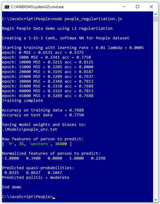
Figure 4-3: L2 Regularization Can Reduce Overfitting and Improve Accuracy

When regularization works properly, model accuracy on the training data is often lower than accuracy on the training data without regularization, but model accuracy on the test data, which is the key metric, is higher.

The underlying math principle is that L2 regularization works by adding a term that penalizes weight values to the error function. The ideas are illustrated by the equations in Figure 4-4.

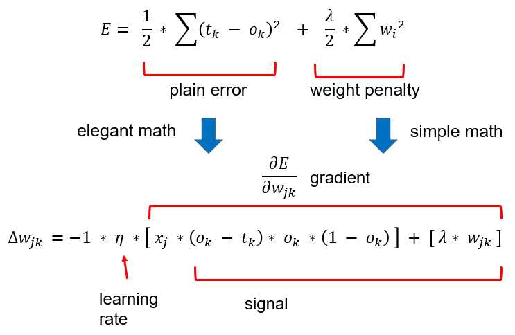
Figure 4-4: Adding a Weight Penalty to Error Changes Weight Deltas

You add a fraction (often called the “L2 regularization constant” and given the lowercase lambda Greek letter) of the sum of the squared weight values to the error. The top-most equation is squared error augmented with the L2 weight penalty: one-half the sum of the squared differences between the target values and the computed output values, plus one-half a constant lambda times the sum of the squared weight values.

During ordinary training, the back-propagation algorithm iteratively adds a weight-delta (which can be positive or negative) to each weight. The weight-delta is a fraction (called the learning rate, usually given lowercase eta Greek symbol, which resembles a script 'n') of the weight gradient. The weight gradient is the calculus derivative of the error function.

To use L2 regularization, you have to add the derivative of the weight penalty. Luckily, this is quite easy. You can see this as the last term in the gradient part of the weight-delta equation.

Let me emphasize that I've abused the formal math notation somewhat, and this explanation is not mathematically one hundred percent accurate. But a thorough, rigorous explanation of the relationship between back-propagation and L2 regularization with all the details would take many pages of messy math.

Although the L2 regularization math concepts are complex, modifying basic back-propagation training to use L2 regularization is surprisingly simple. The program People_regularization.js makes only a few changes to the People_nn.js program.

The definition of class method train() requires a new parameter for the L2 regularization weight term.

  train(trainX, trainY, lrnRate, maxEpochs, lamda)
  {
. . .

I use the misspelled "lamda" rather than "lambda" because lambda is a reserved word in many programming languages. In the train() implementation, the computations for the hidden-to-output gradients and the input-to-hidden gradients have to be changed slightly to add a weight penalty.

  // compute hidden-to-output weight gradients using output signals.
  for (let j = 0; j < this.nh; ++j) {
    for (let k = 0; k < this.no; ++k) {
      hoGrads[j][k] = oSignals[k] * this.hNodes[j];
      hoGrads[j][k] += lamda * this.hoWeights[j][k];  // L2 penalty
    }
  }

. . .    

  // compute input-to-hidden weight gradients using hidden signals.
  for (let i = 0; i < this.ni; ++i) {
    for (let j = 0; j < this.nh; ++j) {
      ihGrads[i][j] = hSignals[j] * this.iNodes[i];
      ihGrads[i][j] += lamda * this.ihWeights[i][j];  // L2 penalty
    }
  }

In short, to add L2 regularization to standard back-propagation, you only need to add two lines of code.

To call the train() method, you just need to add the lambda L2 weighting term.

  // 3. train network
  let lrnRate = 0.01;
  let maxEpochs = 50000;
  let lamda = 0.0005;
  console.log("\nStarting training with learning rate = 0.01 lambda = 0.0005");
  nn.train(trainX, trainY, lrnRate, maxEpochs, lamda);
  console.log("Training complete");

As it turns out, L2 regularization is extremely sensitive to the value used for the lambda weighting term and finding a good value for lambda can be difficult. But when regularization works, it can be highly effective in reducing model overfitting.

Researchers worked out the details of L2 regularization for neural networks in the 1990s. But at the same time, engineers discovered the same basic idea independently, and called the technique “weight decay.” Formal L2 regularization decreases the value of a network's gradients, and then the gradients are used to decrease the magnitude of the network's weights and biases.

Weight decay skips the modification of the gradients and directly reduces the magnitude of the value of weights and biases on each iteration. The weight decay mechanism is much simpler than formal L2 regularization. The computation of gradients is done exactly as it is without regularization. Then during weight and biases updates, after each update, the magnitude is decreased. For example, the following.

// update input-to-hidden weights and apply weight decay.
for (let i = 0; i < this.ni; ++i) {
  for (let j = 0; j < this.nh; ++j) {
    let delta = -1.0 * lrnRate * ihGrads[i][j];
    this.ihWeights[i][j] += delta;
    this.ihWeights[i][j] *= lamda;  // decrease weight (different from L2 lambda).
  }
}

Somewhat unfortunately, both L2 regularization and weight decay regularization usually use a parameter named lambda as the scaling constant. However, by looking at the code, you can see that the lambda values are used very differently. The point is, if you're using a neural network library, the meaning of a regularization lambda can vary (although larger values of lambda ultimately reduce weights more than smaller values).

A technique that is closely related to L2 regularization is called max norm constraint. The idea is to put a fixed limit on the magnitude of all weights. For example, immediately after updating each weight and bias in the train() method, you check to see if the new weight value is greater than a fixed threshold value (perhaps 10.0) or less than the corresponding threshold value (-10.0), and if so, you adjust the weight to the threshold value.

Dropout

Dropout is an advanced technique used to reduce the likelihood of neural network overfitting. The technique sounds strange: on each training iteration, a portion (typically something like 0.50 or 0.20) of the network's hidden nodes are randomly dropped, meaning the training algorithm acts as if the nodes that have been selected to be dropped don't exist.

Dropout can be used for classification problems or regression problems. It can be used in conjunction with other techniques such as regularization, or it can be used by itself.

The screenshot in Figure 4-5 shows an example of training using dropout. The goal is to predict a person's political leaning (conservative, moderate, or liberal) from their sex, age, geo-region (eastern, western, or central), and annual income.

Because dropout effectively trains with just some of the hidden nodes, in general you want to use more hidden nodes than you'd use without dropout. The dropout demo uses twice as many hidden nodes (50 versus 25) as the nondropout demo. Additionally, in many situations, you may have to adjust the values of the learning rate and maximum-epochs to get good results.

Without dropout, the final training and test classification accuracies (shown in Figure 4-1) were 96.25% and 52.50%, but with dropout, the final accuracies are 65.63% and 75.00%. So, the model's accuracy on the training data is quite a bit worse, but the accuracy on the test data, which is the key metric, is significantly better.

The theory behind dropout is shown in Figure 4-6. The neural network has three input nodes, four hidden nodes, and two output nodes, and so does not correspond to the demo program. When using back-propagation, on each training iteration, each node-to-node weight (indicated by the blue arrows) and each node bias (indicated by the green arrows) are updated slightly.

With dropout, on each training iteration, a proportion of the hidden node is randomly selected to be dropped. Then the drop nodes essentially don't exist, so they don't take part in the computation of output node values, or in the computation of the weight and bias updates. In the diagram, if hidden nodes are 0-indexed, then hidden nodes [1] and [2] are selected as drop nodes on this training iteration.

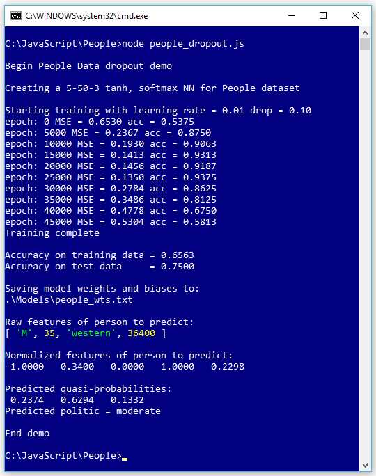
Figure 4-5: Neural Network Dropout Demo Run

Drop nodes aren't physically removed; instead, they are virtually removed by having any code that references them ignore the nodes. In this case, in addition to hidden nodes [1] and [2], the six input-to-hidden weights that terminate in the drop nodes are ignored. And the four hidden-to-output node weights that originate from the drop nodes are ignored.

It's not immediately obvious why dropout reduces overfitting. In fact, the effectiveness of dropout is not fully understood. One notion is that dropout essentially selects random subsets of neural networks, and then averages them together, giving a more robust final result. Another notion is that dropout prevents hidden nodes from relying on other hidden nodes (called coadaptation).

The dropout technique became well known in 2015 following the publication of a research paper. The paper presented a complex mechanism for implementing dropout, which involved many logic branches and code modification to both the training method and the forward-pass evaluation method.

The complex implementation of dropout was used for several years, until engineers noticed that the key ideas of dropout could be implemented in a much simpler way. This simpler technique for dropout implementation is called inverted dropout.

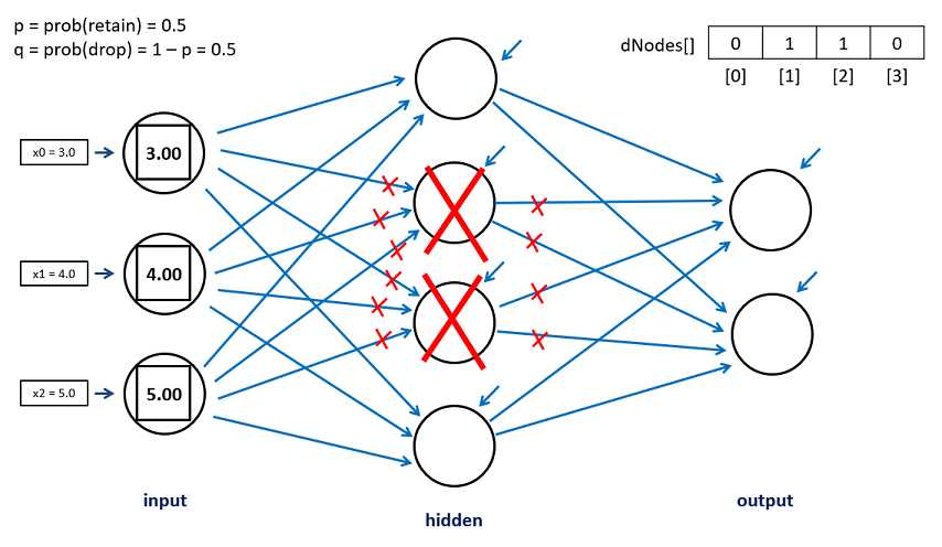
Figure 4-6: The Dropout Mechanism in Theory, but Not in Practice

There are several minor implementation variations that can be used for inverted dropout. The demo modifies the basic train() method by adding a parameter dropProb (drop probability) that controls how many hidden nodes to drop.

  train(trainX, trainY, lrnRate, maxEpochs, dropProb)
  {
    let keepProb = 1.0 - dropProb
    let keepNodes = U.vecMake(this.nh, 0.0);

    let hoGrads = U.matMake(this.nh, this.no, 0.0);
. . .

The numeric vector keepNodes tracks if a hidden node is marked for dropping (value = 0) or not (value = 1). An alternative is to use a vector dropNodes with reversed values, but keepNodes is more convenient programmatically. Another alternative is to use a JavaScript boolean type array instead of a numeric vector.

In the train() method, inside the for-loop that iterates through each training item, a new set of nodes to drop (or equivalently, keep) is determined for each training item.

  for (let ii = 0; ii < n; ++ii) {  // each item
    // select hidden nodes to drop.
    for (let j = 0; j < this.nh; ++j) {
      let p = this.rnd.next();

      if (p < dropProb) {
        keepNodes[j] = 0;  // this is a node to drop.
      }
      else {
        keepNodes[j] = 1;  // keep the node.
      }
    }

Immediately after calling the forward-pass eval() method, dropout is applied.

  let X = trainX[idx];
  let Y = trainY[idx];

  this.eval(X);  // output stored in this.oNodes.
  // apply inverted dropout.
  for (let j = 0; j < this.nh; ++j) {
    if (keepNodes[j] == 0) {
      this.hNodes[j] = 0.0;
    }
    else {
      this.hNodes[j] /= keepProb;
    }
  }

Hidden nodes that have been selected to be dropped have their values overwritten with 0.0, and nodes that aren't dropped have their values scaled larger by dividing by keepProb, the complement of the drop probability. Because keepProb is always less than 1.0, dividing by keepProb always increases a node value. For example, suppose a node's value is 0.90 and dropProb is 0.20; then keepProb is 0.80 and 0.90 / 0.80 = 1.125. Scaling the values of nondrop nodes larger compensates for the drop nodes not contributing to the final output node values, because the drop node values are 0.0.

A call to the train() method with a 10% probability of dropping each hidden node looks like the following.

dropProb = 0.10;
nn.train(trainX, trainY, lrnRate, maxEpochs, dropProb);  // use dropout

Notice that by setting the value of dropProb to 0.0, you get normal back-propagation training without dropout. Also note that the exact number of hidden nodes that will be dropped on each training iteration will likely vary. For example, with 50 hidden nodes, on average 0.10 * 50 = 5 nodes will be dropped. But the exact number of nodes dropped can be between 0 and 50.

The dropout technique was created mostly to deal with overfitting in deep neural networks with many hidden layers and hundreds or even thousands of nodes in each layer. But when used carefully, dropout can improve the prediction accuracy of neural networks with a single hidden layer.

It is possible to apply dropout to input nodes. This technique is most often effective when training data has many predictor variables. A closely related technique is to add random noise to input values. This technique is called jittering.

Train-validate-test

The train-validate-test (TVT) technique can be used to reduce the likelihood of model overfitting. Model overfitting often occurs if a neural network is trained too long. Briefly, instead of splitting your data into a training set and a test set, you split your data into three sets: a training set (typically about 70% of the data), a validation set (often about 15% of the data), and a test set (about 15% of the data).

You use the training data as usual, but every few epochs, you compute and display the error and accuracy of the current model on the validation data. By observing how the model deals with the validation data, you can sometimes see when model overfitting is starting to occur, and then stop training before reaching the max epochs limit.

After training, you compute the error and accuracy of the model on the test data as usual, to get a rough estimate of how the model will perform on new, previously unseen data. The main principle of train-validate-test is shown in the graph in Figure 4-7.

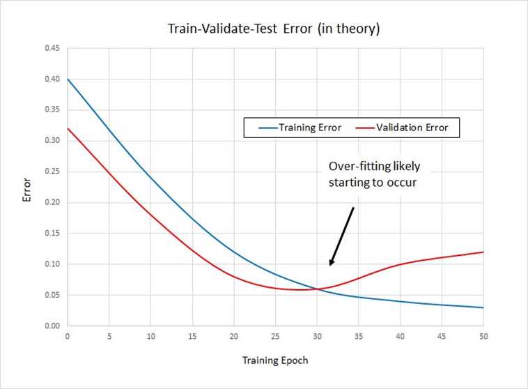
Figure 4-7: Train-Validate-Test in Theory

The blue line represents error on the training data. That error will tend to decrease steadily the longer the network is trained. The red line represents error on the validation data. Initially error will decrease, but at some point, overfitting will start to occur and error on the validation data will start to increase. This can indicate when to stop training.

Unfortunately, there are two reasons why train-validate-test often does not work well. First, you must use valuable labeled data for validation rather than for training. Second, the actual graph of training and validation error is rarely as smooth as shown in Figure 4-7. Instead, the error values for training and validation error often jump around wildly, making it very difficult to determine when overfitting is starting to occur.

The screenshot in Figure 4-8 shows an example of train-validate-test. The goal is to predict a person's political leaning (conservative, moderate, or liberal) from their sex, age, geo-region (eastern, western, or central), and annual income.

The demo program has a total of 240 labeled data items and uses three files: People_train.txt has 160 items, People_validate.txt has 40 items, and People_test.txt has 40 items. The data is synthetic and was generated programmatically.

During training, the demo program computes and displays error and classification prediction accuracy on both the training and validation data. In several runs of the program using 50,000 training epochs, the error and accuracy metrics that were being displayed suggested that overfitting was starting to occur at somewhere between 1,000 and 2,000 epochs. After a bit of experimentation, a value of 1,600 epochs was used to generate the results shown in Figure 4-8.

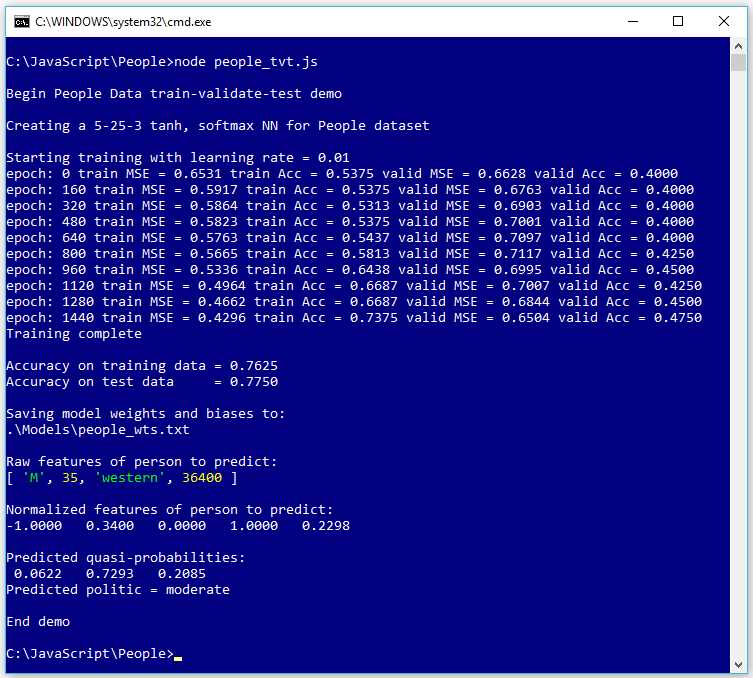
Figure 4-8: Train-Validate-Test Demo

Without train-validate-test, the final training and test classification accuracies (shown in Figure 4-1) were 96.25% and 52.50%, but by using train-validate-test to limit the number of training epochs, the final accuracies are 76.25% and 77.50%. So the model's accuracy on the training data is somewhat worse, but the accuracy on the test data, which is the key metric, is significantly better.

Implementing train-validate-test is straightforward. In the main() function you load the three files into six matrices.

  let trainX = U.loadTxt(".\\Data\\people_train.txt", "\t", [0,1,2,3,4]);
  let trainY = U.loadTxt(".\\Data\\people_train.txt", "\t", [5,6,7]);

  let validX = U.loadTxt(".\\Data\\people_validate.txt", "\t", [0,1,2,3,4]);
  let validY = U.loadTxt(".\\Data\\people_validate.txt", "\t", [5,6,7]);

  let testX = U.loadTxt(".\\Data\\people_test.txt", "\t", [0,1,2,3,4]);
  let testY = U.loadTxt(".\\Data\\people_test.txt", "\t", [5,6,7]);

In the train() method, you compute and display error and accuracy on the training and validation data every few epochs.

      if (epoch % freq == 0) {
        let trainMSE = this.meanSqErr(trainX, trainY).toFixed(4);
        let trainAcc = this.accuracy(trainX, trainY).toFixed(4);
        let validMSE = this.meanSqErr(validX, validY).toFixed(4);
        let validAcc = this.accuracy(validX, validY).toFixed(4);

        let s1 = "epoch: " + epoch.toString();
        let s2 = " train MSE = " + trainMSE.toString();
        let s3 = " train Acc = " + trainAcc.toString();
        let s4 = " valid MSE = " + validMSE.toString();
        let s5 = " valid Acc = " + validAcc.toString();

        console.log(s1 + s2 + s3+ s4 + s5);
      }

Determining when overfitting is starting to occur is part art and part science, as the saying goes. There have been attempts to design algorithms and code that programmatically determine when overfitting is starting to occur, but these efforts have not succeeded very often.

Using train-validate-test is sometimes called early stopping. However, early stopping is a general term that can be used to describe any technique to halt training before reaching the max-epochs value.

Questions

1. Suppose you want to predict political party using this tiny set of training data:

Age Sex     IQ   Party
----------------------------------------------
46  male    120  independent
24  female  100  democrat
38  male    116  republican

1. Normalize the Age values using min-max normalization.
2. Encode the Sex values using -1 +1 encoding.
3. Normalize the IQ values using z-score normalization (note: mean = 112.0, sd = 8.64).
4. Encode the Party values using one-hot / 1-of-N encoding.