Binary Classification

A binary classification problem is one where the goal is to predict a discrete value that can be one of just two possible values. For example, you might want to predict the sex of a person (male or female) based on predictor variables such as age, occupation, annual income, and so on. Somewhat surprisingly, the techniques used for neural binary classification are quite a bit different than those used for neural multiclass classification, where the variable to predict can be one of three or more possible values.

The screenshot in Figure 6-1 shows a demo of neural network binary classification. The goal of the program is to predict if a patient has heart disease (0 = no, 1 = yes) based on 13 predictor variables such as age, sex, blood pressure, and so on.

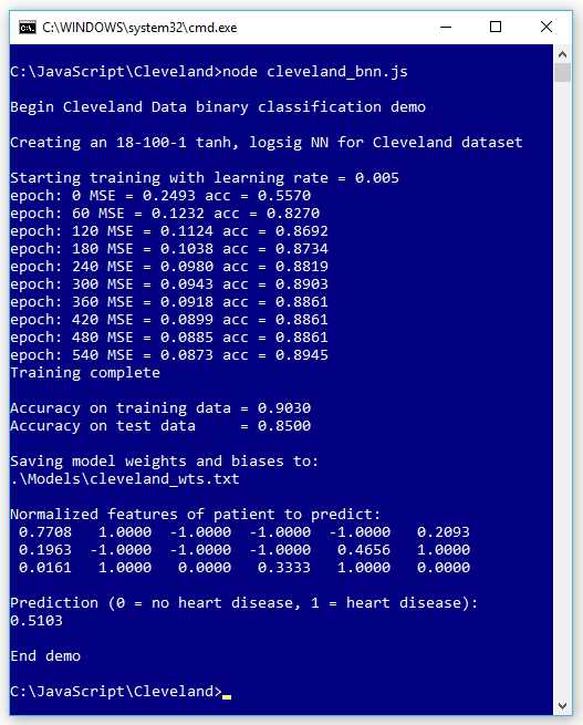
Figure 6-1: Neural Binary Classification

The demo creates an 18-100-1 neural network. The raw training data has 13 predictor variables, but after normalization and encoding, there are 18 values.

The most common technique for neural binary classification is to encode the two possible values to predict as 0 or 1 and use a single output node and coerce the value to be in the range [0.0, 1.0]. If the output value is less than 0.5, then the prediction is class 0; otherwise (if the output value is greater than 0.5), the prediction is class 1.

The number of hidden nodes, 100 in the demo, is a hyperparameter that must be determined by trial and error. The demo uses a learning rate of 0.005 and 600 training epochs (both values are hyperparameters).

The demo program uses the well-known Cleveland Heart Disease data set. The raw data has 303 items, but six items have a missing value, leaving 297 items. The raw data was randomly split into a 237-item set (approximately 80% of the data) for training, and a 60-item set for testing.

The training data has six numeric predictor variables, three binary predictor variables, and four categorical predictor variables. The dependent variable was encoded as 0 = no heart disease and 1 = heart disease. The numeric predictors were min-max normalized. The binary predictors were -1 +1 encoded. The categorical predictors were 1-of-(N-1) encoded. The test data was normalized and encoded using the normalization parameters and encoding scheme from the training data.

After training, the model scored 90.30% accuracy on the training data (214 out of 237 correct) and 85.00% accuracy on the test data (51 out of 60 correct).

The demo program concluded by making a prediction for a new, previously unseen patient. The output of the model is 0.5130, and because that value is greater than 0.5, the prediction is class 1, which is a prediction that the patient has heart disease.

Understanding the Cleveland data set

The demo program uses the Cleveland Heart Disease data set, a well-known classification benchmark data set for statistics and machine learning. The raw data looks like the following.

56.0,  1,  2,  120.0,  236.0,  0,  0,  178.0,  0,  0.8,  1,   3,   3,   0
62.0,  0,  4,  140.0,  268.0,  0,  2,  160.0,  0,  3.6,  3,   1,   6,   3
63.0,  1,  4,  130.0,  254.0,  0,  1,  147.0,  0,  1.4,  2,   2,   ?,   2
53.0,  1,  1,  140.0,  203.0,  1,  2,  155.0,  1,  3.1,  3,   0,   7,   1
[0]   [1] [2]  [3]     [4]    [5] [6]  [7]    [8]  [9]  [10] [11] [12] HD

The first 13 values on each line are the predictor values. The last value is 0 to 4, where 0 indicates no heart disease, and 1 to 4 indicate heart disease of some kind. Predictor [0] is patient age (numeric). Predictor [1] is a sex (0 = female, 1 = male). Predictor [2] is categorical chest pain type encoded as 1 to 4.

Predictor [3] is blood pressure (numeric). Predictor [4] is cholesterol (numeric). Predictor [5] is a related to blood sugar (0 = low, 1 = high). Predictor [6] is categorical electrocardiographic result encoded as (0, 1, 2). Predictor [7] is maximum heart rate (numeric). Predictor [8] is a Boolean for angina (0 = no, 1 = yes). Predictor [9] is ST ("S-wave, T-wave") graph depression.

Predictor [10] is a categorical ST metric encoded as (1, 2, 3). Predictor [11] is a categorical count of colored fluoroscopy vessels encoded as (0, 1, 2, 3). Predictor [12] is a categorical value related to thalassemia encoded as (3, 6, 7).

Because the Cleveland Heart Disease data set has 13 dimensions, it's not possible to easily visualize it in a two-dimensional graph. But you can get a rough idea of the data from the partial graph in Figure 6-2. The graph shows just patient age and blood pressure for the first 160 items of the full data set.

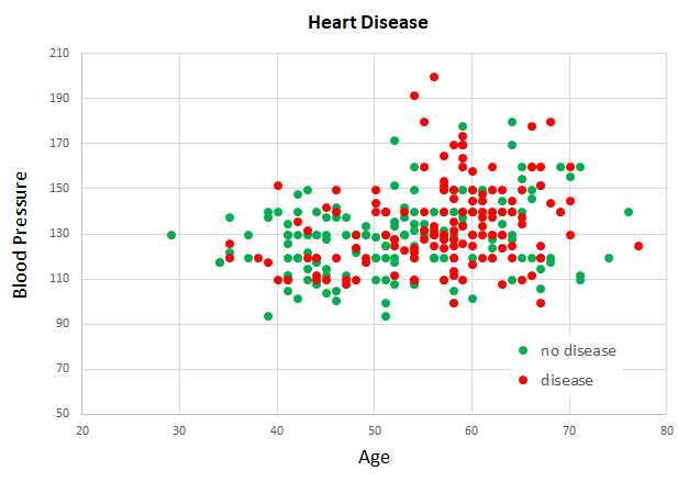
Figure 6-2: Partial Graph of the Cleveland Data Set

As you can see from the graph, it's not possible to get a good prediction model using a simple linear technique like logistic regression or a base support vector machine model.

The Cleveland data set demo program

The complete code for the demo program shown running in Figure 6-1 is presented in Code Listing 6-1. The demo assumes there is a top-level directory named JavaScript that contains subdirectories named Utilities and Cleveland. The Utilities directory contains the Utilities_lib.js library file. The Cleveland directory contains the demo program Cleveland_bnn.js file and subdirectories named Data and Models. The Data directory contains the files Cleveland_train.txt and Cleveland_test.txt. The Models directory is used to store trained model weights and biases values.

Code Listing 6-1: The Cleveland Data Demo Program

All of the control logic is contained in a top-level main() function. Program execution begins by loading the training and test data into memory.

  // 1. load data
  // raw data has 13 predictor values such as age, sex, BP, ECG.
  // normalized and encoded data has 18 values.
  // value to predict: 0 = no heart disease, 1 = heart disease.

  let trainX = U.loadTxt(".\\Data\\cleveland_train.txt", "\t", [0,1,2,3,4,
    5,6,7,8,9,10,11,12,13,14,15,16,17]);
  let trainY = U.loadTxt(".\\Data\\cleveland_train.txt", "\t", [18]);

  let testX = U.loadTxt(".\\Data\\cleveland_test.txt", "\t", [0,1,2,3,4,
    5,6,7,8,9,10,11,12,13,14,15,16,17]);
  let testY = U.loadTxt(".\\Data\\cleveland_test.txt", "\t", [18]);
. . .

The loadTxt() function is contained in file Utilities_lib.js, which is located in the Utilities directory. Notice that the data files are tab-delimited. Next, a neural network is created.

  // 2. create network
  console.log("\nCreating an 18-100-1 tanh, logsig NN for Cleveland dataset");
  let seed = 0;
  let nn = new NeuralNet(18, 100, 1, seed);
. . .

A neural network classifier has a single output node and uses logistic sigmoid activation on that node to force the value to be between 0.0 and 1.0. Technically, the output value represents the probability of class 1. Next, the network is trained.

  // 3. train network
  let lrnRate = 0.005;
  let maxEpochs = 600;
  console.log("\nStarting training with learning rate = 0.005 ");
  nn.train(trainX, trainY, lrnRate, maxEpochs);
  console.log("Training complete");
. . .

The demo uses standard online training. Options include using dropout, using regularization, using momentum, and using the batch or mini-batch techniques.

Next, the trained mode is evaluated.

  // 4. evaluate model
  let trainAcc = nn.accuracy(trainX, trainY);
  let testAcc = nn.accuracy(testX, testY);

  console.log("\nAccuracy on training data = " +
    trainAcc.toFixed(4).toString());

  console.log("Accuracy on test data     = " +
    testAcc.toFixed(4).toString());
. . .

With binary classification, you have to be careful interpreting accuracy when your data is highly skewed towards one of the two classes. For example, if you have a set of training data with 1,000 items and 950 of those items are class 0, then you could get 95% accuracy by predicting class 0 regardless of input values.

Next, the trained model's weights and biases are saved to a text file.

  // 5. save model
  let fn = ".\\Models\\cleveland_wts.txt";
  console.log("\nSaving model weights and biases to: ");
  console.log(fn);
  nn.saveWeights(fn);
. . .

The demo program concludes by making a prediction for a new, previously unseen patient.

  // 6. use trained model
  let unknownNorm = [0.7708, 1, -1, -1, -1, 0.2093, 0.1963, -1, -1, -1,
    0.4656, 1, 0.0161, 1, 0, 0.3333, 1, 0];
  let prediction = nn.eval(unknownNorm);

  console.log("\nNormalized features of patient to predict: ");
  U.vecShow(unknownNorm, 4, 6);  // 4 decimals, 6 values per line

  console.log("\nPrediction (0 = no heart disease, 1 = heart disease): ");
  console.log(prediction[0].toFixed(4).toString());
. . .

The demo program normalizes and encodes the new person item offline. An alternative that is useful when making many predictions is to write a problem-specific function to normalize and encode. For example, using such a function might look like the following.

let unknownRaw = [36, 0, etc.];  // 36 years old, female, etc.
let unkNorm = normAndEncode(unknownRaw);
let predicted = nn.eval(unkNorm);

Note that a program-defined function to normalize and encode raw data needs to know the normalization parameters, such as min and max if min-max normalization is used, and the encoding scheme for non-numeric data. Writing a function to normalize and encode raw data is not difficult conceptually, but it is often very time-consuming.

The demo program leaves it up to the user to interpret the output value. You could add code to display the output value in user-friendly form.

  if (prediction[0] < 0.5) {
    console.log("patient is predicted to have low chance of heart disease");
  }
  else {
    console.log("patient is predicted to have high chance of heart disease");
  }

Notice that the output value is stored in a 1´1 matrix rather than in a scalar variable.

Logistic sigmoid activation

A neural network classifier has multiple output nodes and uses softmax activation on the output nodes so that their values sum to 1.0 and can be loosely interpreted as probabilities. In back-propagation training, the derivative of the function used for output layer activation is used to compute the gradients, which in turn are used to update the network's weights and biases.

A neural network for binary classification uses just a single output node and uses the logistic sigmoid function for output layer activation. The logistic sigmoid function is defined as y = 1.0 / (1.0 + exp(-x)). Although it's not at all obvious, the calculus derivative is y' = y * (1 - y). Somewhat surprisingly, this is the same as the derivative of the softmax activation function.

In the method train() for binary classification, the output node signals are computed using these statements.

  // compute output node signals.
  for (let k = 0; k < this.no; ++k) {
    let derivative = (1 - this.oNodes[k]) * this.oNodes[k];  // log-sig
    oSignals[k] = derivative * (this.oNodes[k] - Y[k]);  // E=(t-o)^2
  }

The eval() method for binary classification is the following.

. . .
  // compute output node before activation.
  for (let k = 0; k < this.no; ++k) {
    for (let j = 0; j < this.nh; ++j) {
      oSums[k] += this.hNodes[j] * this.hoWeights[j][k];
    }
    oSums[k] += this.oBiases[k];
  }

  for (let k = 0; k < this.no; ++k) {
    this.oNodes[k] = U.logSig(oSums[k]);  // logistic sigmoid activation
  }
 
To summarize, to perform binary classification, you encode the variable to predict as 0 or 1. Your neural network has a single output node, uses logistic sigmoid activation for the output layer, and y * (1 - y) as the derivative term for the output node signals.

Binary cross entropy

When creating a neural network for binary classification, you can use mean squared error as in the demo program, or you can use binary cross-entropy error. Regular cross-entropy error compares a set of predicted probabilities with a set of correct probabilities. With only one output node, there are no sets of probabilities to compare, so a special form of cross entropy is used.

Suppose t is a target probability value and y is a predicted output probability (a value between 0.0 and 1.0). For just two values, the cross-entropy error equation is CEE = -[log(y) * t + log(1-y) * (1-t)]. But in neural binary classification, the target is always a 1 or a 0.

If t = 1, the log(1-y) * (1-t) term drops out, leaving just -log(y). If t = 0, the log(y) * t term drops out, leaving just log(1-y). To compute binary cross-entropy error for a neural network, if the target is 1, use -log(y), and if the target is 0, use -log(1-y).

Suppose you have just three training items with the following target and computed output values.

target   computed output
------------------------
  1         0.80
  0         0.30
  1         0.90

The three binary cross entropy terms are -log(0.80) = 0.223, -log(0.70) = 0.357, and -log(0.9) = 0.105, and therefore, the mean binary cross-entropy error is (0.223 + 0.357 + 0.105) / 3 = 0.228.

A possible implementation is the following.

  meanBinCrossEntErr(dataX, dataY)  // for binary classification problems.
  {
    let sum = 0.0;

    for (let i = 0; i < dataX.length; ++i) {  // each data item
      let oupt = this.eval(dataX[i]);

      if (dataY[i] == 1) {  // target is 1
        sum += Math.log(oupt);
      }
      else {  // target is 0
        sum += Math.log(1.0 - oupt);
      }
    }

    return -1 * sum / dataX.length;
  }

Recall that back-propagation training does not explicitly compute error; instead, back-propagation uses the calculus derivative of the error/loss function. For mean squared error, the relevant code is the following.

  // compute output node signals.
  for (let k = 0; k < this.no; ++k) {
    let derivative = (1 - this.oNodes[k]) * this.oNodes[k];  // logsig
    oSignals[k] = derivative * (this.oNodes[k] - Y[k]);  // E=(t-o)^2
  }     

  // now compute hidden-to-output weight gradients using output signals.

But if you assume binary cross-entropy error instead of mean squared error, many of the terms cancel each other out and, in one of the most surprising results in all of machine learning (well, surprising to me, anyway), the computation of the output node signals reduces to the following.

  // compute output node signals.
  for (let k = 0; k < this.no; ++k) {
    oSignals[k] = this.oNodes[k] - Y[k];  // E = binary cross entropy
  }     

In words, everything cancels out, leaving just the computed output value and the target value. Quite remarkable.

When training, it's good practice to print the current error and accuracy every few epochs so that you can see when training is not working. For binary classification problems, regardless of whether you assume mean squared error or binary cross-entropy error, you can compute and display either error term because both will indicate when training is not working. Mean squared error is slightly easier to interpret because the value will always be between 0.0 and 1.0.

The two-node technique for binary classification

By far the most common approach to neural network binary classification is to use a single output node scaled with logistic sigmoid activation and target values of 0 or 1. An alternative is to encode target values as (1, 0) or (0, 1) and use two output nodes scaled with softmax activation. The problem becomes a standard multiclass classification problem. Research results comparing the one-node and two-node techniques are inconclusive, in my opinion.

Questions

1. Suppose you have just three training items with the following target and computed output values.

target   computed output
------------------------
  1         0.70
  0         0.20
  1         0.60

1. Compute the mean squared error.
2. Compute the mean binary cross-entropy error.