Value Prediction

Quick intro

In the previous chapter, we explored the core aspects of ML.NET. We used Model Builder to create a data classification scenario using binary classification to perform spam detection using a small dataset. By doing that, we could create a model, consume and test it, and explore the behind-the-scenes code generated by Model Builder to train and build the machine learning pipeline.

In this chapter, we’ll follow a similar process, but we will work with a value prediction Model Builder scenario this time. We’ll also create the model, consume and test it, and explain the generated code. We’ll then be able to compare both scenarios' differences and how the code differs. So, with that said, let’s begin.

Dataset explanation

The dataset we’ll use throughout this chapter is a slightly modified version of the Boston House Prices dataset. The Boston House prices dataset aims to predict the median price (in 1972) of a house in one of 506 towns or villages near Boston. Each of the 506 data items has 12 predictor variables—11 numeric and 1 Boolean.

If you download and look at the original dataset, you’ll notice that although the file has the .csv file extension, the values are not comma-separated but are instead separated by spaces. You’ll also see the original file doesn’t have headers (it doesn’t include the column names, even though the columns are described on the webpage).

I edited the original dataset by replacing the white spaces with commas and adding headers (column names) on the first row. The edited dataset, which you can find in my GitHub repository, is the one we will use. So, please download it.

Dataset columns

Let’s review the dataset's columns and what each one represents, so you can understand what the values mean when you look at the dataset:

·     CRIM: Indicates the crime rate by town per capita.

·     ZN: Reflects the proportion of residential land for lots over 25,000 sq. ft.

·     INDUS: Specifies the proportion of nonretail business acres per town.

·     CHAS: Is the Charles River variable (1 if tract bounds river; 0 otherwise).

·     NOX: Indicates the nitric oxide concentration (parts per ten million).

·     RM: Indicates the average number of rooms per dwelling.

·     AGE: Indicates the proportion of owner-occupied units built before 1940.

·     DIS: Specifies the distances to five employment centers in Boston.

·     RAD: Indicates the accessibility to highways.

·     TAX: Indicates the full-value property-tax rate per $10,000.

·     PTRATIO: Indicates the pupil-teacher ratio by town.

·     MEDV: Represents the median value of owner-occupied homes in thousands of dollars.

The goal is to use the Value Prediction scenario using the modified dataset to predict the value of MEDV based on the values represented by the other columns.

Creating the model

So, with Visual Studio open, let’s create a new console application. Click the File menu, click on New, and then on Project.

Select the Console App project option and then click Next. You’ll then be shown the following screen, where you can specify the project's name. I’ve renamed the project ValuePredict (which I suggest you use) and set the project’s Location.

Figure 3-a: The “Configure your new project” Screen (Visual Studio)

To continue to the following screen, click Next, and as for the Framework option, any of the options available is fine—I’ll be using .NET 6.0 (Long Term Support). Once done, click Create.

At this point, the project has been created and the next step is to add the model. To do that, within the Solution Explorer, click on ValuePredict to select the app, then right-click, choose Add, and then click Machine Learning Model.

Figure 3-b: Adding a Machine Learning Model (ML.NET)

I’ll give it the name ValuePredictionModel and then click Add. Once done, you’ll notice that the ValuePredictionModel.mbconfig file has been added to the Visual Studio project, and the Model Builder UI appears.

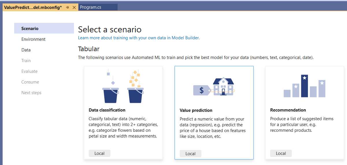
Figure 3-c: Model Builder—Select a scenario (Value prediction)

Let’s continue by choosing the Value prediction scenario. To do that, click on the Local button below the Value prediction description.

Figure 3-d: Model Builder—Select training environment

To continue, all we have to do is click Next step. At this stage, we will add the modified dataset. We can do that by clicking Browse, selecting the housing.csv file, and then clicking Open.

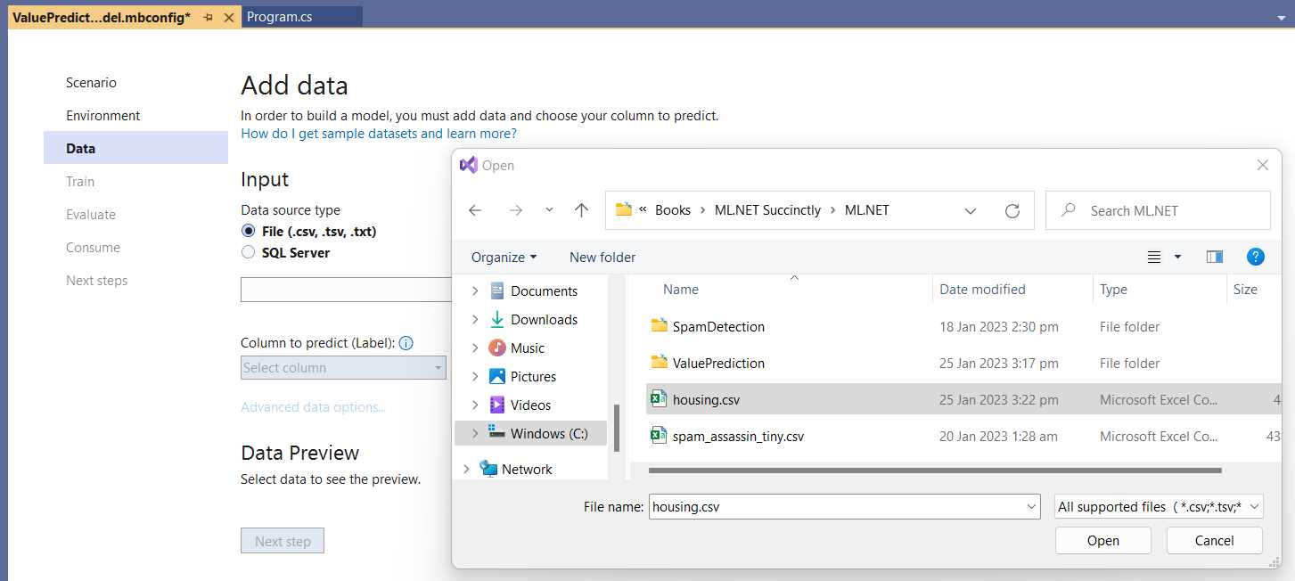
Figure 3-e: Model Builder—Add data (Selecting housing.csv)

Once that has been done, the data will be imported and visible within the Data Preview table.

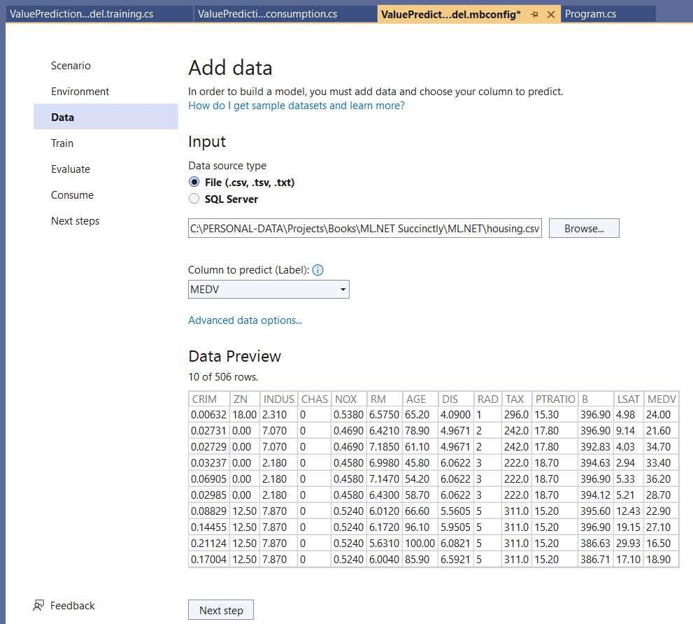
Figure 3-f: Model Builder—Add data (Data Added)

From the Column to predict (Label) dropdown, select the MEDV column, which indicates the house prices.

With that done, click Next step to continue with the training step. To train the model, click Start training. Once the model has been trained, you should see an overview of the Training results.

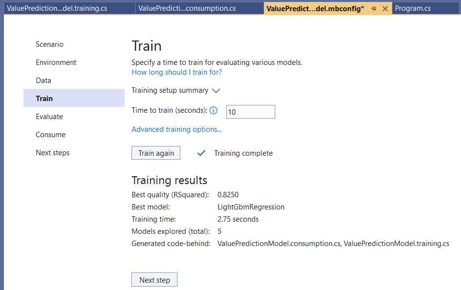
Figure 3-g: Model Builder—Train (Training results)

Notice that the algorithm chosen by Model Builder as the best option for the training data used by this model is LightGbmRegression, based on decision trees.

Next, you can evaluate the model. To do that, click Next step; the Evaluate step will be shown.

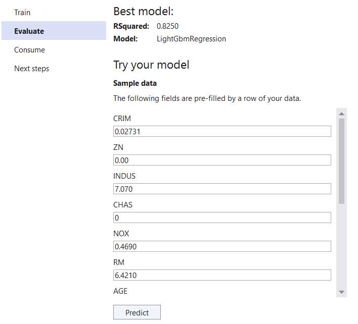
Figure 3-h: Model Builder–Evaluate (Try your model)

Given that we are using a dataset with multiple columns, we are presented with all the input columns available, which we can use to test our newly created model. The test input values are prefilled with data inferred by Model Builder. To view all the test values, scroll down the list. When ready, click Predict—this will display the prediction results.

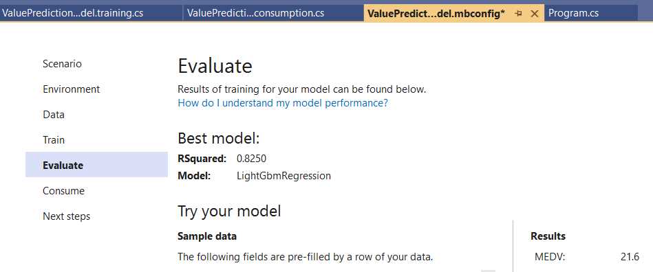
Figure 3-i: Model Builder—Evaluate (Try your model with Results)

Once the prediction value is available, we can continue by clicking on Next step to get ready to consume the model.

Figure 3-j: Model Builder—Consume

With this scenario, we will do the same thing we did with the spam detection example we previously created: copy the code snippet and consume it directly from the project we already started. But before we copy the code snippet generated by Model Builder, let’s go to Solution Explorer and open Program.cs. The code looks as follows.

Code Listing 3-a: Program.cs

Let’s replace the preceding code with the following code that uses the code snippet generated by Model Builder and consumes the model. The bold line is not part of the generated code snippet. I’ve added it manually to see the model’s prediction result (result.Score), which indicates the predicted house price.

Code Listing 3-b: Program.cs (Modified)

We should see the following output if we run the program by clicking the run button within Visual Studio.

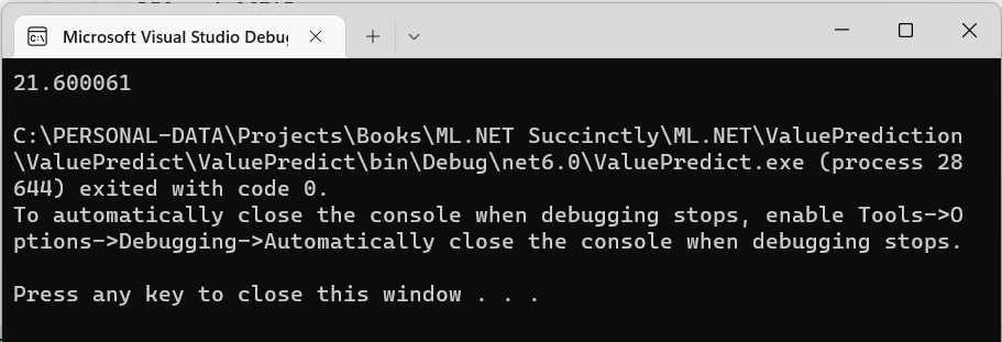
Figure 3-k: The Program Running—Microsoft Visual Studio Debugger

Notice that the output value (21.6) is the same one Model Builder displayed when evaluating the model. Now that we can consume the model correctly, let’s switch to Solution Explorer and look at the files that Model Builder generated and added to the project.

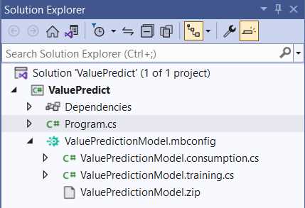
Figure 3-l: The ValuePredictionModel Files Generated by Model Builder—Solution Explorer

As you can see, Model Builder generated three files, ValuePredictionModel.consumption.cs, ValuePredictionModel.training.cs, and ValuePredictionModel.zip.

ValuePredictionModel.consumption.cs

Let’s open this file within Solution Explorer to look at the generated code in detail.

Code Listing 3-c: ValuePredictionModel.consumption.cs

The code begins with the using statements that reference the libraries imported and used, Microsoft.ML and Microsoft.ML.Data.

Following that, we find the ValuePredictionModel class, declared as partial, given that it resides in both ValuePredictionModel.*.cs files. Within the class, we find the ModelInput and ModelOutput classes. The ModelInput class contains the values used as input by the model, and the ModelOutput class contains the output values. The ModelInput and ModelOutput classes contain properties corresponding to the dataset columns we previously explored.

However, the main difference between both classes is that the ModelOutput class has the Features and Score properties that are specific to the model’s prediction results.

Then, we find MLNetModelPath, which points to the location where the model’s metadata is found.

Next is the PredictEngine variable, an instance of Lazy<PredictionEngine<ModelInput, ModelOutput>>.

To create the instance, the constructor receives as a first parameter a lambda function that instantiates the engine: () => CreatePredictEngine(), and the second parameter (true) indicates whether the instance can be used by multiple threads (thread-safe).

Next, we have the Predict method, which is used for making predictions based on the model, as follows. The Predict method receives as a parameter a ModelInput instance (input), which represents the input data for the model. The predicted value (PredictEngine.Value) is assigned to the predEngine variable. The result of invoking the predEngine.Predict method is returned by the Predict method.

Then, we find the CreatePredictEngine method, which, as its name implies, creates the prediction engine instance.

private static PredictionEngine<ModelInput, ModelOutput> CreatePredictEngine()

{

  var mlContext = new MLContext();

  ITransformer mlModel = mlContext.Model.Load(MLNetModelPath, out var _);

  return mlContext.Model.

    CreatePredictionEngine<ModelInput, ModelOutput>(mlModel);

}

This method first creates an instance of MLContext, which is assigned to the mlContext variable.

Following that, the model is loaded, which is done by invoking the Load method from mlContext.Model, to which the model’s metadata path (MLNetModelPath) is passed as a parameter.

The out var _ parameter represents the modelInputSchema. The Load method returns the model loaded as an object (mlModel).

The prediction engine (PredictEngine) is created using the CreatePredictionEngine method from mlContext.Model, to which the object model (mlModel) is passed as a parameter.

Overall, ValuePredictionModel.consumption.cs contains the generated code for creating the prediction engine and invoking it—thus, allowing the model consumption.

As you have seen, the pattern used by Model Builder to programmatically generate the code for ValuePredictionModel.consumption.cs is almost identical to the code generated for the spam detection use case we previously explored (TestModel.consumption.cs). The only difference is the properties of the ModelInput and ModelOutput classes, which differ between both use cases.

With ValuePredictionModel.consumption.cs, the predicted result is assigned to the Score property of the ModelOutput class, contrary to TestModel.consumption.cs, where a target column (label) was used.

ValuePredictionModel.training.cs

Let’s move on to the Solution Explorer and open the ValuePredictionModel.training.cs file.

Code Listing 3-d: ValuePredictionModel.training.cs

Let’s explore each part of the code individually to understand what is happening. First, we find the using statements—the Microsoft.ML.Trainers.LightGbm namespace is referenced besides Microsoft.ML. The Microsoft.ML.Trainers.LightGbm namespace contains the methods used by ML.NET to implement the LightGbm algorithm.

Then, within the partial ValuePredictionModel class, we find the RetrainPipeline method. The RetrainPipeline method is responsible for retraining the model once the pipeline has been built. This method has two parameters, an instance of MLContext and the training data (trainData) of type IDataView (used as the input and output of transforms).

The RetrainPipeline method returns an object that implements the ITransformer interface responsible for transforming data within an ML.NET model pipeline. It builds the model’s pipeline using different transforms and algorithms.

The call to the pipeline.Fit method retrains the model (using trainData), returning the retrained model.

On the other hand, the BuildPipeline method receives as a parameter an MLContext instance and returns an object that implements the IEstimator<ITransformer> interface.

The pipeline is created using transformations that are added using mlContext.Transforms. The first step is to replace any missing values from the model’s input, which is done by calling the ReplaceMissingValues method from mlContext.Transforms.

The ReplaceMissingValues method receives an InputOutputColumnPair array. This array indicates how each model’s input columns map to the model’s output columns. In this case, the input and output columns have the same names. So, invoking InputOutputColumnPair(@"CRIM", @"CRIM") indicates that the CRIM input column maps to the CRIM output column, and so on.

In short, the ReplaceMissingValues method prepares the input data and ensures there aren’t missing values for processing. You can specify how to replace missing values, such as using the mean value in a column. The demo code uses the default technique based on the column's data type. In any event, the Boston dataset has no missing values.

Like we saw within the TestModel.training.cs file, the ReplaceMissingValues method is the first step in creating the pipeline. Following that, we find a series of chained calls to the Append method that add more steps to the pipeline.

In the initial Append step, we can see the Concatenate method from mlContext.Transforms being invoked. As you can see, all the dataset columns are concatenated, except the MEDV column (which is the value we want the model to predict), to produce the Features property.  This indicates which input columns will be considered to make the prediction (thus, the name Features).

The next step in the pipeline specifies the algorithm to use for training the model, which is done by invoking the LightGbm method from mlContext.Regression.Trainers.

For the LightGbm algorithm, we need to specify a set of configuration options—these are passed as an instance of LightGbmRegressionTrainer.Options.

The great thing about Model Builder is that it can find the best values for the algorithm settings. If we were to do this manually, it would require a lot of trial and error, using different values and seeing which would give the best prediction result. Notice that one of the settings passed to the algorithm is a GradientBooster.Options instance, which specifies that the algorithm should implement gradient boosting.

Once the last Append method has been chained, the training pipeline is ready and returned by the BuildPipeline method.

ValuePredictionModel.training vs. TestModel.training

As previously seen, ValuePredictionModel.consumption.cs and TestModel.consumption.cs are essentially the same in terms of what they do and achieve. But that’s not the case with the ValuePredictionModel.training.cs and TestModel.training.cs files, which are very different. Let’s first explore these differences visually.

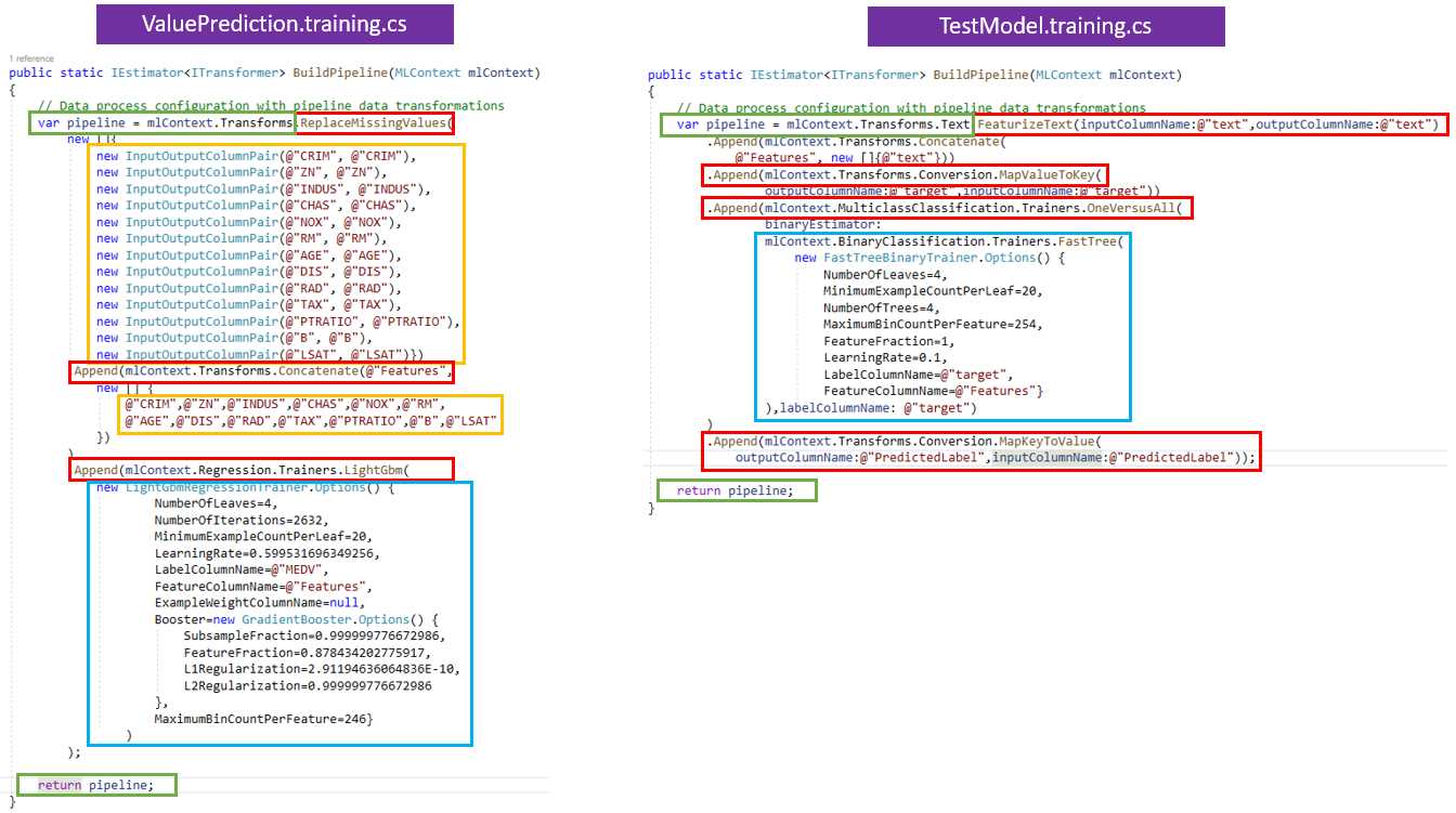
Figure 3-m: ValuePredictionModel.training.cs vs. TestModel.training.cs

I’ve included the BuildPipeline method for both files because they differ, as seen in the preceding image; however, the RetrainPipeline method is the same for both files. Given that the differences between the files reside only within the BuildPipeline method, I’ve highlighted these differences with different colors.

I have highlighted in red the main differences in how the pipeline is built. We can see the number of steps required to create the pipeline within the ValuePrediction.training.cs file is one less than the number of steps needed to create a pipeline within the TestModel.training.cs file.

In light green, I have highlighted the common features of the BuildPipeline method for both files. Essentially, the only commonality is that both declare and return the pipeline variable.

The algorithm to train each of these models is highlighted in light blue. The algorithm used by the TestModel.training.cs file is FastTree, and the one used by ValuePrediction.training.cs is LightGbm.

Highlighted in light yellow, we can see the data and feature preparation steps used only within the ValuePrediction.training.cs file.

By looking at these differences, we can conclude that the differences between these two models, in terms of code, are only three. These differences are down to how the pipelines are built, the data preparation steps, and the algorithm used to train each model.

Summary

We have seen throughout this chapter that a value prediction model solves a different type of prediction problem than a data classification model. Both scenarios are based on using tabular data as input to create a prediction.

Essentially, the main differences between them reside in the type of data used (such as the number of input columns), the steps used in creating each pipeline, and the algorithm applied to generate the prediction.

Nevertheless, the ways both models are retrained and consumed resemble each other, so we can almost certainly assume that this will likely be the pattern for different prediction scenarios.

In the following chapter, we will explore a different scenario using nontabular input data and see whether we can corroborate the exciting findings from this chapter.