Basic Syntax

All the work you do in MATLAB will involve the use of variables, so we will begin by looking at the ways in which variables are declared and manipulated.

Just like any other programming language, MATLAB has different operators for doing different things, so we will take a look at the ones that matter most. Don’t worry, there aren’t that many of those. Next, we will talk about flow control—things like if and switch statements and for and while loops. We will finish the chapter with a discussion of exception handling.

Working with Variables

When working with any kind of computation in MATLAB, we make use of variables. A variable is essentially a storage location: it can store a numeric value, a character, an array, or can refer to a more advanced construct such as a function or structure.

Variables typically have names. A variable name in MATLAB has to start with a letter followed by a zero, more letters, digits, or underscores. Any name is valid except names that have been taken by MATLAB keywords (e.g., if or for).

There is one variable in MATLAB that you simply cannot avoid meeting: it’s called ans and it stores the result of the last calculation, assuming that the calculation actually returned a value that was not specifically assigned to another variable. Indeed, it’s also possible to assign the ans variable, though this is perhaps not the best idea, as it’s likely to be overwritten at any moment.

In addition to ans, you can specify the name of the variable to assign a value to:

It’s also possible to assign multiple variables at once. The function that is responsible for this is called deal, and is used to define, on a single line, an assignment of either same or different values to multiple variables. Variables must be declared in square brackets, separated by a comma:

Variable Data Import and Export

The state of all the variables in your workspace can be saved into a special kind of file that stores MATLAB Formatted Data. This file has a .mat extension, and essentially contains a snapshot of the workspace. To work with these files using the Command Window, you can use the save and load functions. These can be used without parameters (in which case the file name used is matlab.mat), or you can specify your own filename. You can also use save and load to store individual variables in MAT data files.

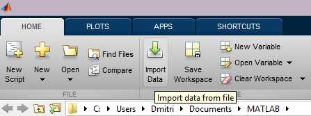
In addition to MATLAB Formatted Data, you can also import files in known data formats—not just CSV and the like, but also image data, movies, and many other formats. You can find the Import Data button on the ribbon:

The import process can be customized via the UI (for example, you can tell MATLAB to correctly interpret a particular date/time format), and you can also generate the code that actually performs the import, which is super-useful if you want to share both your script files and data.

Basic Operators

Since MATLAB is a programming language, basic mathematical operations (addition, subtraction, multiplication, and division) use the predictable +, -, * and / operators. Just as in ordinary math, round parentheses can be used to group operations. Square brackets and curly braces are reserved for other uses (numeric and cell arrays, respectively).

For taking a to the power of b, MATLAB uses the ^ (hat or circumflex) symbol. MATLAB also has the (somewhat bizarre) back-division operator \ (backslash). This operator has a special meaning for matrices, but for “scalar” values, a\b simply means the same as b/a. It is probably not a good idea to use this operator for this purpose, unless you deliberately want to obfuscate your code.

Each of the aforementioned operators also has an elementwise equivalent prefixed by a dot (e.g., .+, ./ and so on). We will discuss elementwise operators later on in the book.

The single = (equals) operator is used for assigning values, e.g. meaningOfLife = 42. If you want to compare two values, you use the == operator instead or, if you want to check that the values are different, use ~=, which is the equivalent of the ≠ sign. Speaking of comparisons, MATLAB also supports the < and > operators as well as the “or equal” <= and >= counterparts (equivalent to ≤ and ≥ in math notation). Note that comparisons yield a 0 or a 1 indicating false and true respectively, but the result is not an integer, but a single-byte logical value:

Values of logical type can be treated as numeric values for the purposes of calculations, but any numeric operation on them will yield a double value.

It’s also important to note that you can supply numeric values to constructs that expect logical values (e.g., if statements). In this case, MATLAB treats the value of 0 to mean false and any other value to mean true. I wouldn’t recommend using this feature, though, as it can lead to difficult-to-spot errors.

Now let’s talk about the , (comma) and ; (semicolon) operators. MATLAB, unlike many programming languages, does not require you to terminate your statements with the semicolon. However, if you do not, the resulting value of a calculation will be printed to the command window. If you do terminate the statement with a semicolon, though, nothing gets printed to the command window:

The comma operator is used to separate parameters to a function, but it also has a more obscure use case—when you want to separate several statements on a single line, but you do want command window output. In this case, simply separate the statements with a comma instead:

The % (percent) operator is used to create comments, and is particularly useful in scripts. Everything following the % sign on a particular line is ignored by MATLAB for purposes of execution, but the operator does have special uses when it comes to publishing scripts (discussed later).

Finally there is the ! (exclamation point) operator. This operator is used to issue commands to the operating system and, as you can imagine, its function depends on the OS you’re running. For example, on Windows, we can issue a command that lists the contents of the current directory:

Note: MATLAB actually has its own dir function, so you can call it without the exclamation mark and get a similar (but not identical) result.

Flow Control

Let us begin with the if statement—this statement lets you check a condition (e.g., the result of a comparison) and perform an operation depending on whether the result is true or false (remember that in MATLAB these are denoted by 1 and 0 respectively). For example, if we have a temperature reading and we need to determine whether or not it’s hot outside, we can write the following check:

This piece of code checks the value of t, and if it is greater than 100, outputs the line ‘hot’ to the command window. We can add additional checks to the if statement, checking for example if it is cold. To do this, we add an elseif clause:

Now, if the first check fails, the second check is performed. If neither are successful, though (for example, t=50), nothing happens. Now, if we want to execute some other piece of code if none of the conditions in our if statement are true, we can add an else clause:

A temperature measurement is a continuous value, but if we want to investigate a discrete set of values—say, a country’s dialing codes—we might want to use another kind of control flow structure called a switch statement. This statement tries to match a variable’s content against a set of discrete values. For example, to determine the country name from the country code we can write:

If the country code is 44, we print uk, if it is 46 we print sweden, but if it is equal to some other value that we failed to match against, we print unknown. Note that there is no need to explicitly terminate a case in a switch statement.

Quite often, we want to cycle through a set of values, performing an operation on each. For example, let us try iteratively adding up numbers from 1 to 500 (not the best way of doing things, but good enough for a demonstration). To cycle through the values, we use a for loop:

In this example, the variable i takes on all values in the 1 to 500 range, and at each iteration, this value is added to sum.

A while loop is similar to the for loop, with the difference that instead of iterating a set of values, it checks a condition and keeps executing while the condition holds. For example, the following code generates and outputs random values between 0 and 1 while they are less than 0.7:

As soon as a value greater than or equal to 0.7 is generated, the v < 0.7 check fails and we exit the while loop.

Sometimes you might be somewhere in the middle of the loop and want to cut the execution short. In this case, you can execute a break statement, which will take you out of the loop and continue executing just after the end statement:

The above rule is deliberately made to run forever by providing a 1 (true) in the condition, but we break out of a loop as soon as the sum of two random values exceeds 1.0. Similarly, had we wanted to avoid printing the x and y values inside this loop, we could replace the break keyword with continue, which would simply take us to the start of the loop.

Exception Handling

Anytime you do something MATLAB doesn’t like, you end up with an exception. An exception is an indication that something went wrong and MATLAB doesn’t know how to deal with it. For example, a division by zero is not an exception, since MATLAB can just give you the inf constant, but if you try to read a variable that doesn’t exist, there’s no way to gracefully handle this, so MATLAB just fails with an error message.

After an exception is generated, all other statements that follow it will not execute. To avoid this situation, I can actually try to catch this exception if I think that it might happen. The way to do it is to place the code where exceptions can occur in a try-catch block:

If I execute this, assuming that the variable abc does not exist, I get the following output:

It’s worth explaining what’s going on above. When we catch the exception, it gets stored in a variable (in our case, it’s called e). The exception is itself a class object (we discuss classes in Chapter 7) with detailed information about the error:

As you can see, the exception has a type MException, and it has several fields, including an identifier, the actual message (that’s what we printed to the command window) as well as the stack (which happens to be an array of structs), which tells you who threw the exception and where:

It’s also possible to rethrow exceptions and, needless to say, you can create and throw exceptions of your own using the error function.