Neural Network Classification

---

Introduction

Neural networks are software systems that loosely model biological neurons and synapses. Neural network classification is one of the most interesting and sophisticated topics in all of machine learning. One way to think of a neural network is as a complex mathematical function that accepts one or more numeric inputs and generates one or more numeric outputs.

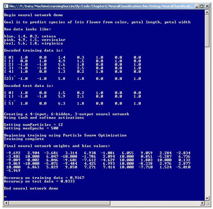
Figure 5-a: Neural Network Classification Demo

A good way to get an understanding of what neural networks are is to examine the screenshot of a demo program in Figure 5-a. The goal of the demo is to create a model that can predict the species of an iris flower based on the flower's color, petal length, and petal width.

The source data set has 30 items. The first three data items are:

blue, 1.4, 0.3, setosa
pink, 4.9, 1.5, versicolor
teal, 5.6, 1.8, virginica

The predictor variables (also called independent variables, features, and x-data) are in the first three columns. The first column holds the iris flower's color, which can be blue, pink, or teal. The second and third columns are the flower's petal length and width. The fourth column holds the dependent variable, species, which can be setosa, versicolor, or virginica.

Note: the demo data is an artificial data set patterned after a famous, real data set called Fisher's Iris data. Fisher's real data set has 150 items and uses sepal length and sepal width instead of color. (A sepal is a green, leaf-like structure).

Because neural networks work internally with numeric data, the categorical color values and species must be encoded as numeric values. The demo assumes this has been done externally. The first three lines of encoded data are:

[ 0]   1.0     0.0     1.4     0.3     1.0     0.0     0.0
[ 1]   0.0     1.0     4.9     1.5     0.0     1.0     0.0
[ 2]  -1.0    -1.0     5.6     1.8     0.0     0.0     1.0

The species values are encoded using what is called 1-of-N dummy encoding. Categorical data value setosa maps to numeric values (1, 0, 0), versicolor maps to (0, 1, 0), and virginica maps to (0, 0, 1). There are several other, less common, encoding schemes for categorical dependent variables.

The independent variable color values are encoded using 1-of-(N-1) effects encoding. Color blue maps to (1, 0), pink maps to (0, 1), and teal maps to (-1, -1). Although there are alternatives, in my opinion the somewhat unusual looking 1-of-(N-1) effects encoding is usually the best approach to use for categorical predictor variables.

Using the 30-item source data, the demo program sets up a 24-item training set, used to create the neural network model, and a 6-item test set, used to estimate the accuracy of the model when presented with new, previously unseen data.

The demo program creates a four-input-node, six-hidden-node, three-output-node neural network. The number of input and output nodes, four and three, are determined by the structure of the encoded data. The number of hidden nodes for a neural network is a free parameter and must be determined by trial and error.

There are dozens of variations of neural networks. The demo program uses the most basic form, which is a fully-connected, feed-forward architecture, with a hyperbolic tangent (often abbreviated tanh) hidden layer activation function and a softmax output layer activation function. Activation functions will be explained shortly.

Behind the scenes, a 4-6-3 neural network has a total of (4)(6) + 6 + (6)(3) + 3 = 51 numeric values, called weights and biases. These weights determine the output values for a given set of input values. Training a neural network is the process of finding the best set of values for the weights and biases, so that when presented with the training data, the computed outputs closely match the known outputs. Then, when presented with new data, the neural network uses the best weights found to make predictions.

There are several techniques that can be used to train a neural network. By far, the most common technique is called back-propagation. In fact, back-propagation training is so common that people new to neural networks sometimes assume it is the only training technique. The demo program uses an alternative technique called particle swarm optimization (PSO).

Basic PSO training requires just two parameter values. The demo program uses 12 particles, and sets a maximum training loop count of 500. These parameters will be explained shortly.

After the neural network is trained using PSO, the demo program displays the values of the 51 weights and biases that define the model. The demo computes the accuracy of the final model on the training data, which is 91.67% (22 out of 24 correct), and the accuracy on the test data (83.33%, five out of six correct). The 83.33% figure can be interpreted as a rough estimate of how well the final neural network model would predict the species of new, previously unseen iris flowers.

Understanding Neural Network Classification

The process by which a neural network computes output values is called the feed-forward mechanism. Output values are determined by the input values, the hidden weights and bias values, and two activation functions. The process is best explained with a concrete example. See the diagram in Figure 5-b.

The diagram shows a fully connected 3-4-2 dummy neural network, which does not correspond to the demo problem. Although the neural network appears to have three layers of nodes, the first layer, the input layer, is normally not counted, so the neural network in the diagram is usually called a two-layer network.

Each arrow connecting one node to another represents a weight value. Each hidden and output node also has an arrow that represents a special weight called a bias. The neural network's three input values are { 1.0, 5.0, 9.0 }, and the two output values are { 0.4886, 0.5114 }.

The feed-forward process begins by computing the values for the hidden nodes. Each hidden node value is an activation function applied to the sum of the products of input node values and their associated weight values, plus the node's bias value. For example, the top-most hidden node's value is computed as:

hidden[0] sum = (1.0)(0.01) + (5.0)(0.05) + (9.0)(0.09) + 0.13
                        = 0.01 + 0.25 + 0.81 + 0.13
                        = 1.20

hidden[0] value  = tanh(1.20)
                          = 0.8337 (rounded)

The dummy neural network is using tanh, the hyperbolic tangent function. The tanh function accepts any real value and returns a result that is between -1.0 and +1.0. The main alternative to the tanh function for hidden layer activation is the logistic sigmoid function.

Figure 5-b: The Neural Network Feed-Forward Mechanism

Next, each output node is computed in a similar way. Preliminary output values for all nodes are computed, and then the preliminary values are combined, so that all output node values sum to 1.0. In Figure 5-b, the two output node preliminary output values are:

output[0] prelim = (.8337)(.17) + (.8764)(.19) + (.9087)(.21) + (.9329)(.23) + .25
                          = 0.9636

output[1] prelim = (.8337)(.18) + (.8764)(.20) + (.9087)(.22) + (.9329)(.24) + .26
                          = 1.0091

These two preliminary output values are combined using an activation function called the softmax function to give the final output values like so:

output[0] = e^0.9636 / (e^0.9636 + e^1.0091)
               = 2.6211 / (2.6211 + 2.7431)
               = 0.4886

output[1] = e^1.0091 / (e^0.9636 + e^1.0091)
               = 2.7431 / (2.6211 + 2.7431)
               = 0.5114
The point of using the softmax activation function is to coerce output values to sum to 1.0 so that they can be interpreted as the probabilities of the y-values.

For the dummy neural network in Figure 5-b, there are two output nodes, so suppose those nodes correspond to predicting male or female, where male is dummy-encoded as (1, 0) and female is encoded as (0, 1). If the output values (0.4886, 0.5114) are interpreted as probabilities, the higher probability is in the second position, and so the output values predict (0, 1), which is female.

Binary neural network classification, where there are two output values, is a special case that can, and usually is, treated differently from problems with three or more output values. With just two possible y-values, instead of using softmax activation with two output nodes and dummy encoding, you can use the logistic sigmoid function with just a single output node and 0-1 encoding.

The logistic sigmoid function is defined as f(z) = 1.0 / (1.0 + e^-z). It accepts any real-valued input and returns a value between 0.0 and 1.0. So if two categorical y-values are male and female, you would encode male as 0 and female as 1. You would create a neural network with just one output node. When computing the value of the single output node, you'd use the logistic sigmoid function for activation. The result will be between 0.0 and 1.0, for example, 0.6775. In this case, the computed output, 0.6775, is closer to 1 (female) than to 0 (male) so you'd conclude the output is female.

Another very common design alternative applies to any type of neural network classifier. Instead of using separate, distinct bias values for each hidden and output node, you can consider the bias values as special weights that have a hidden, dummy, constant associated input value of 1.0. In my opinion, treating bias values as special weights with invisible 1.0 inputs is conceptually unappealing, and more error-prone than just treating bias values as bias values.

Demo Program Overall Structure

To create the demo, I launched Visual Studio and selected the new C# console application template. After the template code loaded into the editor, I removed all using statements at the top of the source code, except for the single reference to the top-level System namespace. In the Solution Explorer window, I renamed file Program.cs to the more descriptive NeuralProgram.cs, and Visual Studio automatically renamed class Program to NeuralProgram.

The overall structure of the demo program, with a few minor edits to save space, is presented in Listing 5-a. In order to keep the size of the example code small, and the main ideas as clear as possible, the demo program omits normal error checking.

Listing 5-a: Neural Network Classification Demo Program Structure

All the neural network classification logic is contained in a single program-defined class named NeuralNetwork. All the program logic is contained in the Main method. The Main method begins by setting up 24 hard-coded (color, length, width, species) data items in an array-of-arrays style matrix:

static void Main(string[] args)

{

  Console.WriteLine("\nBegin neural network demo\n");

  Console.WriteLine("Raw data looks like: \n");

  Console.WriteLine("blue, 1.4, 0.3, setosa");

  Console.WriteLine("pink, 4.9, 1.5, versicolor");

  Console.WriteLine("teal, 5.6, 1.8, virginica \n");

  double[][] trainData = new double[24][];

  trainData[0] = new double[] { 1, 0, 1.4, 0.3, 1, 0, 0 };

  trainData[1] = new double[] { 0, 1, 4.9, 1.5, 0, 1, 0 };

  trainData[2] = new double[] { -1, -1, 5.6, 1.8, 0, 0, 1 };

. . .

The demo program assumes that the color values, blue, pink, and teal, have been converted either manually or programmatically to 1-of-(N-1) encoded form, and that the three species values have been converted to 1-of-N encoded form.

For simplicity, the demo does not normalize the numeric petal length and width values. This is acceptable here only because their magnitudes, all between 0.2 and 7.0, are close enough to the -1, 0, and +1 values of the 1-of-(N-1) encoded color values such that neither feature will dominate the other. In most situations, you should normalize your data.

Next, the demo creates six hard-coded test data items:

double[][] testData = new double[6][];

testData[0] = new double[] { 1, 0, 1.5, 0.2, 1, 0, 0 };

testData[1] = new double[] { -1, -1, 5.9, 2.1, 0, 0, 1 };

testData[2] = new double[] { 0, 1, 1.4, 0.2, 1, 0, 0 };

testData[3] = new double[] { 0, 1, 4.7, 1.6, 0, 1, 0 };

testData[4] = new double[] { 1, 0, 4.6, 1.3, 0, 1, 0 };

testData[5] = new double[] { 1, 0, 6.3, 1.8, 0, 0, 1 };

In a non-demo scenario, the training and test data would be programmatically generated from the source data set using a utility method named something like MakeTrainTest or SplitData.

After displaying a few lines of the training and test data using static helper method ShowData, the demo program creates and instantiates a program-defined NeuralNetwork classifier object:

Console.WriteLine("\nCreating a 4-input, 6-hidden, 3-output neural network");

Console.WriteLine("Using tanh and softmax activations \n");

int numInput = 4;

int numHidden = 6;

int numOutput = 3;

NeuralNetwork nn = new NeuralNetwork(numInput, numHidden, numOutput);

There are four input nodes to accommodate two values for the 1-of-(N-1) encoded color, plus the petal length and width. There are three output nodes to accommodate the 1-of-N encoded three species values: setosa, versicolor, and virginica. Determining the number of hidden nodes to use is basically a matter of trial and error.

Next, the neural network is trained:

int numParticles = 12;

int maxEpochs = 500;

Console.WriteLine("Setting numParticles = " + numParticles);

Console.WriteLine("Setting maxEpochs = " + maxEpochs);

Console.WriteLine("\nBeginning training using Particle Swarm Optimization");

double[] bestWeights = nn.Train(trainData, numParticles, maxEpochs);

Console.WriteLine("Training complete \n");

Console.WriteLine("Final neural network weights and bias values:");

ShowVector(bestWeights, 10, 3, true);

The demo program uses particle swarm optimization (PSO) for training. There are many variations of PSO, but the demo uses the simplest form, which requires only the number of virtual particles and the maximum number of iterations for the main optimization loop.

After training completes, the best weights found are stored in the NeuralNetwork object. For convenience, the training method also explicitly returns the best weights found. The 51 weights and bias values are displayed using helper method ShowVector. The demo program does not save the weight values that define the model, so you might want to write a SaveWeights method.

The demo program concludes by computing the classification accuracy of the final model:

. . .
  nn.SetWeights(bestWeights);

  double trainAcc = nn.Accuracy(trainData);

  Console.WriteLine("\nAccuracy on training data = " + trainAcc.ToString("F4"));

  double testAcc = nn.Accuracy(testData);

  Console.WriteLine("Accuracy on test data = " + testAcc.ToString("F4"));

  Console.WriteLine("\nEnd neural network demo\n");

  Console.ReadLine();

} // Main

Note that because the best weights found are stored in the NeuralNetwork object, the call to method SetWeights is not really necessary.

The demo program does not use the model to make a prediction for a new data item that has an unknown species. Prediction could look like:

double[] unknown = new double[] { 1, 0, 1.9, 0.5 }; // blue, petal = 1.9, 0.5
nn.SetWeights(bestWeights);
string species = nn.Predict(unknown);
Console.WriteLine("Predicted species is " + species);

Defining the NeuralNetwork Class

The structure of the program-defined NeuralNetwork class is presented in Listing 5-b. Data member array inputs holds the x-values. Member matrix ihWeights holds the input-to-hidden weights. For example, if ihWeights[0][2] is 0.234, then the weight connecting input node 0 to hidden node 2 has value 0.234.

Listing 5-b: The NeuralNetwork Class

Member array hBiases holds the hidden node bias values. Member array hOutputs holds the values of the hidden nodes after the hidden layer tanh function has been applied. After they're computed, these values act as local inputs when computing the output layer nodes.

Member matrix hoWeights holds the hidden-to-output node weights. Member array oBiases holds the bias values for the output nodes. Member array outputs holds the final output node values. Member rnd is a Random object, which is used during the PSO training algorithm.

The NeuralNetwork class has a single constructor. Static helper method MakeMatrix is called by the constructor, and is just a convenience to allocate the ihWeights and hoWeights matrices. The constructor code is simple:

public NeuralNetwork(int numInput, int numHidden, int numOutput)

{

  this.numInput = numInput;

  this.numHidden = numHidden;

  this.numOutput = numOutput;

  this.inputs = new double[numInput];

  this.ihWeights = MakeMatrix(numInput, numHidden);

  this.hBiases = new double[numHidden];

  this.hOutputs = new double[numHidden];

  this.hoWeights = MakeMatrix(numHidden, numOutput);

  this.oBiases = new double[numOutput];

  this.outputs = new double[numOutput];

  this.rnd = new Random(0);

}

Random object rnd is instantiated with a seed value of 0 only because that value gave a representative demo run. You might want to experiment with different seed values.

Method ComputeOutputs implements the feed-forward mechanism. The definition begins:

public double[] ComputeOutputs(double[] xValues)

{

  double[] hSums = new double[numHidden]; // hidden nodes sums scratch array

  double[] oSums = new double[numOutput]; // output nodes sums
. . .

Recall that hidden and output nodes are computed in two steps. First, a sum of products is computed, and then an activation function is applied. Arrays hSums and oSums hold the sum of products. A design alternative is to declare hSums and oSums as class-scope arrays to avoid allocating them on every call to ComputeOutputs. However, if you do this, you'd have to remember to explicitly zero out both arrays inside ComputeOutputs.

Next, ComputeOutputs transfers the x-data parameter values into the class inputs array:

for (int i = 0; i < xValues.Length; ++i) // copy x-values to inputs

  this.inputs[i] = xValues[i];

A very important design alternative is to delete the class inputs array from the NeuralNetwork definition and use the x-data values directly. This saves the overhead of copying values into inputs at the expense of clarity.

Next, the hidden node values are computed using the feed-forward mechanism:

for (int j = 0; j < numHidden; ++j)  // sum of weights * inputs

  for (int i = 0; i < numInput; ++i)

    hSums[j] += this.inputs[i] * this.ihWeights[i][j]; // note +=

for (int i = 0; i < numHidden; ++i)  // add biases

  hSums[i] += this.hBiases[i];

for (int i = 0; i < numHidden; ++i)   // apply activation

  this.hOutputs[i] = HyperTan(hSums[i]);

Here, the hyperbolic tangent function is hard-coded into the class definition. A design alternative is to pass the hidden layer activation function in as a parameter. This gives additional calling flexibility at the expense of significantly increased design complexity.

Helper method HyperTan is defined:

private static double HyperTan(double x)

{

  if (x < -20.0)

    return -1.0; // approximation is correct to 30 decimals

  else if (x > 20.0)

    return 1.0;

  else return Math.Tanh(x);

}

Although you can just call built-in method Math.Tanh directly, the demo checks the input value x first because for small or large values of x, the tanh function returns values that are extremely close to 0.0 or 1.0, respectively.

After computing the hidden node values, method ComputeOutputs computes the output layer node values:

for (int j = 0; j < numOutput; ++j)   // sum of weights * hOutputs

  for (int i = 0; i < numHidden; ++i)

    oSums[j] += hOutputs[i] * hoWeights[i][j];

for (int i = 0; i < numOutput; ++i)  // add biases to input-to-hidden sums

  oSums[i] += oBiases[i];

double[] softOut = Softmax(oSums); // all outputs at once for efficiency

Array.Copy(softOut, outputs, softOut.Length);

Calculating the softmax outputs is a bit subtle. If you refer to the explanation of how softmax works, you'll notice that the calculation requires all the preliminary outputs, so unlike hidden nodes which are activated one at a time, output nodes are activated as a group.

The definition of helper method Softmax is:

private static double[] Softmax(double[] oSums)

{

  // determine max output-sum

  double max = oSums[0];

  for (int i = 0; i < oSums.Length; ++i)

    if (oSums[i] > max) max = oSums[i];

  // determine scaling factor -- sum of exp(each val - max)

  double scale = 0.0;

  for (int i = 0; i < oSums.Length; ++i)

    scale += Math.Exp(oSums[i] - max);

  double[] result = new double[oSums.Length];

  for (int i = 0; i < oSums.Length; ++i)

    result[i] = Math.Exp(oSums[i] - max) / scale;

  return result; // now scaled so that xi sum to 1.0

}

Method Softmax is short, but quite tricky. Instead of computing softmax outputs using the direct definition, method Softmax uses some clever math. The indirect implementation gives the same result as the definition, but avoids potential arithmetic underflow or overflow problems, because intermediate values in the direct-definition calculation can be extremely close 0.0.

Understanding Particle Swarm Optimization

The most common technique to train neural networks is called back-propagation. Back-propagation is based on classical calculus techniques, and is conceptually complex, but relatively simple to implement. The major disadvantage of back-propagation is that it requires you to specify values for two parameters called the learning rate and the momentum. Back-propagation is extraordinarily sensitive to these parameter values, meaning that even a tiny change can have a dramatic impact.

Particle swarm optimization (PSO) also requires parameter values, but is much less sensitive than back-propagation. The major disadvantage of using PSO for training is that it is usually slower than using back-propagation.

PSO is loosely modeled on coordinated group behavior, such as the flocking of birds. PSO maintains a collection of virtual particles where each particle represents a potential best solution to a problem, which, in the case of neural networks, is a set of values for the weights and biases that minimize the error between computed output values and known output values in a set of training data.

Expressed in very high-level pseudo-code, PSO looks like:

initialize n particles to random solutions/positions and velocities
loop until done
  for each particle
    compute a new velocity based on best known positions
    use new velocity to move particle to new position/solution
  end for
end loop
return best solution/position found by any particle

PSO is illustrated in Figure 5-c. In a simple case where a solution consists of two values, like (1.23, 4.56), you can think of a solution as a point on an (x, y) plane. The graph shows two particles. In most situations, there would be many particles. The goal is to minimize the function f(x, y) = 3x² + 3y². The solution is x = y = 0.0, so the problem doesn't really need PSO; the example is intended just to illustrate how PSO works.

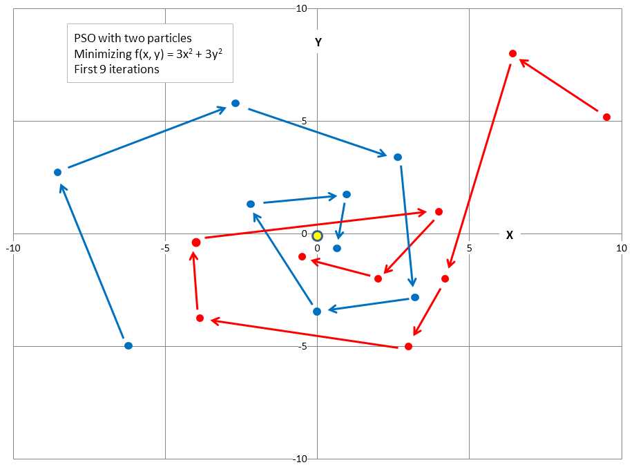
Figure 5-c: Example of Particle Swarm Optimization

The first particle, in the lower left, starts with a randomly generated initial solution of (-6.0, -5.0) and random initial velocity (direction) values that move the particle up and to the left. The second particle, in the upper right, has random initial value (9.5, 5.1) and random initial velocity that will move the particle up and to the left.

The graph shows how each particle moves during the first nine iterations of the main PSO loop. The new position of each particle is influenced by its current direction, the best position found by the particle at any time, and the best position found by any of the particles at any time. The net result is that particles tend to move in a coordinated way and converge on a good, hopefully optimum, solution. In the graph, you can see that both particles quickly got very close to the optimal solution of (0, 0).

In math terms, the PSO equations to update a particle's velocity and position are:

v(t+1) = (w * v(t)) + (c1 * r1 * (p(t) – x(t)) + (c2 * r2 * (g(t) – x(t))

x(t+1) = x(t) + v(t+1)

The position update process is actually much simpler than these equations appear. The first equation updates a particle's velocity. The term v(t+1) means the velocity at time t+1. Notice that v is bold, indicating that velocity is a vector value and has multiple components, such as (1.55, -0.33), rather than being a single scalar value.

The new velocity depends on three terms. The first term is w * v(t). The w factor is called the inertia weight and is just a constant like 0.73 (more on this shortly), and v(t) is the current velocity at time t. The second term is c1 * r1 * (p(t) – x(t)). The c1 factor is a constant called the cognitive (or personal) weight. The r1 factor is a random variable in the range [0, 1), which is greater than or equal to 0 and strictly less than 1. The p(t) vector value is the particle's best position found so far. The x(t) vector value is the particle's current position.

The third term in the velocity update equation is (c2 * r2 * (g(t) – x(t)). The c2 factor is a constant called the social (or global) weight. The r2 factor is a random variable in the range [0, 1). The g(t) vector value is the best known position found by any particle in the swarm so far. Once the new velocity, v(t+1), has been determined, it is used to compute the new particle position x(t+1).

A concrete example will help make the update process clear. Suppose that you are trying to minimize f(x, y) = 3x² + 3y². Suppose a particle's current position, x(t), is (x, y) = (3.0, 4.0), and that the particle's current velocity, v(t), is (-1.0, -1.5). Additionally, assume that constant w = 0.7, constant c1 = 1.4, constant c2 = 1.4, and that random numbers r1 and r2 are 0.5 and 0.6 respectively. Finally, suppose that the particle's current best known position is p(t) = (2.5, 3.6) and that the current global best known position found by any particle in the swarm is g(t) = (2.3, 3.4). Then the new velocity values are:

v(t+1) = (0.7 * (-1.0,-1.5)) + (1.4 * 0.5 * (2.5, 3.6) - (3.0, 4.0)) + (1.4 * 0.6 * (2.3, 3.4) – (3.0, 4.0))
           = (-0.70, -1.05) + (-0.35, -0.28) + (-0.59, -0.50)
           = (-1.64, -1.83)

Now the new velocity is added to the current position to give the particle's new position:

x(t+1) = (3.0, 4.0) + (-1.64, -1.83)
           = (1.36, 2.17)

Recall that the optimal solution is (x, y) = (0, 0). Observe that the update process has improved the old position or solution from (3.0, 4.0) to (1.36, 2.17). If you examine the update process, you'll see that the new velocity is the old velocity (times a weight) plus a factor that depends on a particle's best known position, plus another factor that depends on the best known position from all particles in the swarm. Therefore, a particle's new position tends to move toward a better position based on the particle's best known position and the best known position from all particles.

Training using PSO

The implementation of method Train begins:

public double[] Train(double[][] trainData, int numParticles, int maxEpochs)

{

  int numWeights = (this.numInput * this.numHidden) + this.numHidden +

    (this.numHidden * this.numOutput) + this.numOutput;
. . .

Method Train assumes that the training data has the dependent variable being predicted, iris flower species in the case of the demo, stored in the last column of matrix trainData. Next, relevant local variables are set up:

int epoch = 0;

double minX = -10.0; // for each weight

double maxX = 10.0;

double w = 0.729; // inertia weight

double c1 = 1.49445; // cognitive weight

double c2 = 1.49445; // social weight

double r1, r2; // cognitive and social randomizations

Variable epoch is the main loop counter variable. Variables minX and maxX set limits for each weight and bias value. Setting limits in this way is called weight restriction. In general, you should use weight restriction only with x-data that has been normalized, or where the magnitudes are all roughly between -10.0 and +10.0.

Variable w, called the inertia weight, holds a value that influences the extent a particle will keep moving in its current direction. Variables c1 and c2 hold values that determine the influence of a particle's best known position, and the best known position of any particle in the swarm. The values of w, c1, and c2 used here are ones recommended by research.

Next, the swarm is created:

Particle[] swarm = new Particle[numParticles];

double[] bestGlobalPosition = new double[numWeights];

double bestGlobalError = double.MaxValue;

The definition of class Particle is presented in Listing 5-c.

Listing 5-c: Particle Class Definition

Class Particle is a container class that holds a virtual position, velocity, and error associated with the position. A minor design alternative is to use a structure instead of a class. The demo program defines class Particle inside class NeuralNetwork. If you refactor the demo code to another programming language that does not support nested classes, you'll have to define class Particle as a standalone class.

Method Train initializes the swarm of particles with his code:

for (int i = 0; i < swarm.Length; ++i)

{

  double[] randomPosition = new double[numWeights];

  for (int j = 0; j < randomPosition.Length; ++j)

    randomPosition[j] = (maxX - minX) * rnd.NextDouble() + minX;

  double error = MeanSquaredError(trainData, randomPosition);

  double[] randomVelocity = new double[numWeights];

  for (int j = 0; j < randomVelocity.Length; ++j)

  {

    double lo = 0.1 * minX;

    double hi = 0.1 * maxX;

    randomVelocity[j] = (hi - lo) * rnd.NextDouble() + lo;

  }

  swarm[i] = new Particle(randomPosition, error, randomVelocity,

    randomPosition, error);

  // does current Particle have global best position/solution?

  if (swarm[i].error < bestGlobalError)

  {

    bestGlobalError = swarm[i].error;

    swarm[i].position.CopyTo(bestGlobalPosition, 0);

  }

}

There's quite a lot going on here, and so you may want to refactor the code into a method named something like InitializeSwarm. For each particle, a random position is generated, subject to the minX and maxX constraints. The random position is fed to helper method MeanSquaredError to determine the associated error. A significant design alternative is to use a different form of error called the mean cross entropy error.

Because a particle velocity consists of values that are added to the particle's current position, initial random velocity values are set to be smaller (on average, one-tenth) than initial position values. The 0.1 scaling factor is to a large extent arbitrary, but has worked well in practice.

After a random position and velocity have been created, those values are fed to the Particle constructor. The call to the constructor may look a bit odd at first glance. The last two arguments represent the particle's best position found and the error associated with that position. So, at particle initialization, these best-values are the initial position and error values.

After initializing the swarm, method Train begins the main loop, which uses PSO to seek a set of best weights:

int[] sequence = new int[numParticles]; // process particles in random order

for (int i = 0; i < sequence.Length; ++i)

  sequence[i] = i;

while (epoch < maxEpochs)

{

  double[] newVelocity = new double[numWeights];

  double[] newPosition = new double[numWeights];

  double newError;

  Shuffle(sequence);
  . . .

In general, when using PSO it is better to process the virtual particles in random order. Local array sequence holds the indices of the particles and the indices are randomized using a helper method Shuffle, which uses the Fisher-Yates algorithm:

private void Shuffle(int[] sequence)

{

  for (int i = 0; i < sequence.Length; ++i)

  {

    int ri = rnd.Next(i, sequence.Length);

    int tmp = sequence[ri];

    sequence[ri] = sequence[i];

    sequence[i] = tmp;

  }

}

The main processing loop executes a fixed maxEpochs times. An important alternative is to exit early if the current best error drops below some small value. The code could resemble:

if (bestGlobalError < exitError)

  break;

Here, exitError would be passed as a parameter to method Train or the Particle constructor. The training method continues by updating each particle. The first step is to compute a new random velocity (speed and direction) based on the current velocity, the particle's best known position, and the swarm's best known position:

for (int pi = 0; pi < swarm.Length; ++pi) // each Particle (index)

{

  int i = sequence[pi];

  Particle currP = swarm[i]; // for coding convenience

 

  for (int j = 0; j < currP.velocity.Length; ++j) // each x-value of the velocity

  {

    r1 = rnd.NextDouble();

    r2 = rnd.NextDouble();

    newVelocity[j] = (w * currP.velocity[j]) +

      (c1 * r1 * (currP.bestPosition[j] - currP.position[j])) +

      (c2 * r2 * (bestGlobalPosition[j] - currP.position[j]));

  }

  newVelocity.CopyTo(currP.velocity, 0);

This code is the heart of the PSO algorithm, and it is unlikely you will need to modify it. After a particle's new velocity has been computed, that velocity is used to compute the particle's new position, which represents the neural network's set of weights and bias values:

for (int j = 0; j < currP.position.Length; ++j)

{

  newPosition[j] = currP.position[j] + newVelocity[j]; // compute new position

  if (newPosition[j] < minX) // keep in range

    newPosition[j] = minX;

  else if (newPosition[j] > maxX)

    newPosition[j] = maxX;

}

newPosition.CopyTo(currP.position, 0);

Notice the new position is constrained by minX and maxX, which is essentially implementing neural network weight restriction. A minor design alternative is to remove this constraining mechanism. After the current particle's new position has been determined, the error associated with that position is computed:

newError = MeanSquaredError(trainData, newPosition);

currP.error = newError;

if (newError < currP.bestError) // new particle best?

{

  newPosition.CopyTo(currP.bestPosition, 0);

  currP.bestError = newError;

}

if (newError < bestGlobalError) // new global best?

{

  newPosition.CopyTo(bestGlobalPosition, 0);

  bestGlobalError = newError;

}

At this point, method Train has finished processing each particle, and so the main loop counter variable is updated. A significant design addition is to implement code that simulates the death of a particle. The idea is to kill a particle with a small probability, and then give birth to a new particle at a random location. This helps prevent the swarm from getting stuck at a non-optimal solution at the risk of killing a good particle (one that is moving to an optimal solution).

After the main loop finishes, method Train concludes. The best position (weights) found is copied into the neural network's weight and bias matrices and arrays, using class method SetWeights, and these best weights are also explicitly returned:

. . .

  SetWeights(bestGlobalPosition);  // best position is a set of weights

  double[] retResult = new double[numWeights];

  Array.Copy(bestGlobalPosition, retResult, retResult.Length);

  return retResult;

} // Train

Method SetWeights is presented in the complete demo program source code at the end of this chapter. Notice all the weights and bias values are stored in a single array, which corresponds to the best position found by any particle. This means that there is an implied ordering of the weights. The demo program assumes input-to-hidden weights are stored first, followed by hidden node biases, followed by hidden-to-output weights, followed by output node biases.

Other Scenarios

This chapter presents all the key information needed to understand and implement a neural network system. There are many additional, advanced topics you might wish to investigate. The biggest challenge when working with neural networks is avoiding over-fitting. Over-fitting occurs when a neural network is trained so that the resulting model has perfect or near-perfect accuracy on the training data, but the model predicts poorly when presented with new data. Holding out a test data set can help identify when over-fitting has occurred. A closely related technique is called k-fold cross validation. Instead of dividing the source data into two sets, the data is divided into k sets, where k is often 10.

Another approach for dealing with over-fitting is to divide the source data into three sets: a training set, a validation set, and a test set. The neural network is trained using the training data, but during training, the current set of weights and bias values are periodically applied to the validation data. Error on both the training and validation data will generally decrease during training, but when over-fitting starts to occur, error on the validation data will begin to increase, indicating training should stop. Then, the final model is applied to the test data to get a rough estimate of the model's accuracy.

A relatively new technique to deal with over-fitting is called dropout training. As each training item is presented to the neural network, half of the hidden nodes are ignored. This prevents hidden nodes from co-adapting with each other, and results in a robust model that generalizes well. Drop-out training can also be applied to input nodes. A related idea is to add random noise to input values. This is sometimes called jittering.

Neural networks with multiple layers of hidden nodes are often called deep neural networks. In theory, a neural network with a single, hidden layer can solve most classification problems. This is a consequence of what is known as the universal approximation theorem, or sometimes, Cybenko's theorem. However, for some problems, such as speech recognition, deep neural networks can be more effective than ordinary neural networks.

The neural network presented in this chapter measured error using mean squared error. Some research evidence suggests an alternative measure, called cross entropy error, can generate more accurate neural network models. In my opinion, the research supporting the superiority of cross entropy error over mean squared error is fairly convincing, but the improvement gained by using cross entropy error is small. In spite of the apparent superiority of cross entropy error, the use of mean squared error seems to be more common.

Ordinary neural networks are called feed-forward networks because when output values are computed, information flows from input nodes to hidden nodes to output nodes. It is possible to design neural networks where some or all of the hidden nodes have an additional connection that feeds back into themselves. These are called recurrent neural networks.

Chapter 5 Complete Demo Program Source Code