Logistic Regression Classification

---

Introduction

Machine learning classification is the process of creating a software system that predicts which class a data item belongs to. For example, you might want to predict the sex (male or female) of a person based on features such as height, occupation, and spending behavior. Or you might want to predict the credit worthiness of a business (low, medium, or high) based on predictors such as annual revenue, current debt, and so on. In situations where the class to predict has just two possible values, such as sex, which can be male or female, the problem is called binary classification. In situations where the dependent class has three or more possible values, the problem is called a multiclass problem.

Machine learning vocabulary can vary wildly, but problems where the goal is to predict some numeric value, as opposed to predicting a class, are often called regression problems. For example, you might want to predict the number of points some football team will score based on predictors such as opponent, home field advantage factor, average number of points scored in previous games, and so on. This is a regression problem.

There are many different machine learning approaches to classification. Examples include naive Bayes classification, probit classification, neural network classification, and decision tree classification. Perhaps the most common type of classification technique is called logistic regression classification. In spite of the fact that logistic regression classification contains the word "regression", it is really a classification technique, not a regression technique. Adding to the confusion is the fact that logistic regression classification is usually shortened to "logistic regression," rather than the more descriptive "logistic classification."

The best way to get an understanding of logistic regression classification is to examine the screenshot in Figure 3-a. The goal of the demo program is to predict whether a hospital patient will die or not based on three predictors: age, sex, and the result of a kidney test. Because the class to predict has just two possible values, die or survive, the demo is a binary classification problem.

All classification techniques use the same general approach. They rely on a set of data with known input and output values to create some mathematical equation that predicts the value of the dependent variable based on the independent, or predictor, variables. Then, after the model has been created, it can be used to predict the result for new data items with unknown outputs.

The demo starts with 30 (artificial) data items. The first two items are:

48.00   1  4.40  0
60.00  -1  7.89  1

The dependent variable to predict, Died, is in the last column and is encoded so that 0 represents false, meaning the person survived, and 1 represents true, meaning the person died. For the feature variables, male is encoded as -1 and female is encoded as +1. The first line of data means a 48-year-old female, with a kidney test score of 4.40 survived. The second data item indicates that there was a 60-year-old male with a 7.89 kidney score who died.

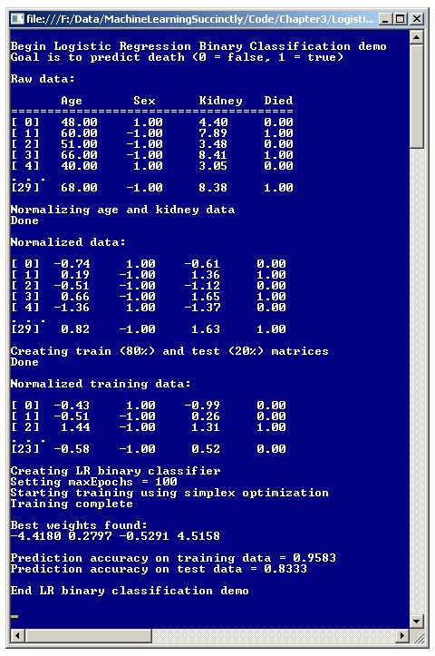
Figure 3-a: Logistic Regression Binary Classification

After reading the data set into memory, the demo program normalizes the independent variables (sometimes called x-data) of age and kidney score. This means that the values are scaled to have roughly the same magnitude so that ages, which have relatively large magnitudes like 55.0 and 68.0, won't overwhelm kidney scores that have smaller magnitudes like 3.85 and 6.33. After normalization, the first two data items are now:

-0.74   1  -0.61  0
0.19  -1   1.36  1

For normalized data, values less than zero indicate below average, and values greater than zero indicate above average. So for the first data item, the age (-0.74) is below average, and the kidney score (-0.61) is also below average. For the second data item, both age (+0.19) and kidney score (+1.36) are above average.

After normalizing the 30-item source data set, the demo program divides the set into two parts: a training set, which consists of 80% of the items (24 items) and a test set, which has the remaining 20% (6 items). The split process is done in a way so that data items are randomly assigned to either the training or test sets. The training data is used to create the prediction model, and the test data is used after the model has been created to get an estimate of how accurate the model will be when presented with new data that has unknown output values.

After the training and test sets are generated, the demo creates a prediction model using logistic regression classification. When using logistic regression classification (or any other kind of classification), there are several techniques that can be used to find values for the weights that define the model. The demo program uses a technique called simplex optimization.

The result of the training process is four weights with the values { -4.41, 0.27, -0.52, and 4.51 }. As you'll see later, the second weight value, 0.27, is associated with the age predictor, the third weight value, -0.52, is associated with the sex predictor, and the last weight value, 4.51, is associated with the kidney score predictor. The first weight value, -4.41, is a constant needed by the model, but is not directly associated with any one specific predictor variable.

After the logistic regression classification model is created, the demo program applies the model to the training and test data, and computes the predictive accuracy of the model. The model correctly predicts 95.83% of the training data (which is 23 out of 24 correct) and 83.33% of the test data (5 out of 6 correct). The 83.33% can be interpreted as an estimate of how accurate the model will be when presented with new, previously unseen data.

Understanding Logistic Regression Classification

Suppose some raw age, sex, and kidney data is { 50.0, -1, 6.0 }, which represents a 50-year-old male with a kidney score of 6.0. Here, the data is not normalized to keep the ideas clear. Now suppose you have four weights: b₀ = -7.50, b₁ = 0.11, b₂ = -0.22, and b₃ = 0.33. One possible way to create a simple linear model would be like so:

Y = b₀ + b₁(50.0) + b₂(-1) + b₃(6.0)
   = -7.50 + (0.11)(50.0) + (-0.22)(-1) + (0.33)(6.0)
   = 0.20

In other words, you'd multiply each input x-value by an associated weight value, sum those products, and add a constant. Logistic regression classification extends this idea by using a more complex math equation that requires a pair of calculations:

Z = b₀ + b₁(50.0) + b₂(-1) + b₃(6.0)
Y = 1.0 / (1.0 + e^-Z)

In other words, for logistic regression classification, you form a linear combination of weights and inputs, call that sum Z, and then feed that result to a second equation that involves the math constant e. The constant e is just a number with value 2.7182818, and it appears in many math equations, in many different fields.

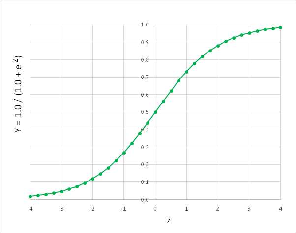
Figure 3-b: The Logistic Sigmoid Function

The function Y = 1.0 / (1.0 + e^-Z) has many important uses in machine learning, and forms the basis of logistic regression classification. The function is called the logistic sigmoid function, or sometimes the log sigmoid, or just the sigmoid function for short. The logistic sigmoid function can accept any Z-value from negative infinity to positive infinity, but the output is always a value between 0 and 1, as shown in Figure 3-b.

This may be mildly interesting, but what's the point? The idea is that if you have some input x-values and associated weights (often called the b-values) and you combine them, and then feed the sum, Z, to the logistic sigmoid function, then the result will be between 0 and 1. This result is the predicted output value.

An example will clarify. As before, suppose that for a hospital patient, some un-normalized age, sex, and kidney x-values are { 50.0, -1, 6.0 }, and suppose the b-weights are b₀ = -7.50, b₁ = 0.11, b₂ = -0.22, and b₃ = 0.33. And assume that class 0 is "die is false" and class 1 is "die is true".

The logistic regression calculation goes like so:

Z = b₀ + b₁(50.0) + b₂(-1) + b₃(6.0)
   = 0.20

Y = 1.0 / (1.0 + e^-Z)
   = 1.0 / (1.0 + e^-0.20)
   = 0.5498

The final predicted output value (0 or 1) is the one closest to the computed output value. Because 0.5498 is closer to 1 than to 0, you'd conclude that dependent variable "died" is true. But if the y-value had been 0.3333 for example, because that value is closer to 0 than to 1, you'd conclude "died" is false. An equivalent, but slightly less obvious, interpretation is that the computed output value is the probability of the 1-class.

Now if you have many training data items with known results, you can compute the accuracy of your model-weights. So the problem now becomes, how do you find the best set of weight values? The process of finding the set of weight values so that computed output values closely match the known output values for some set of training data is called training the model. There are roughly a dozen major techniques that can be used to train a logistic regression classification model. These include techniques such as simple gradient descent, back-propagation, particle swarm optimization, and Newton-Raphson. The demo program uses a technique called simplex optimization.

Demo Program Overall Structure

To create the demo, I launched Visual Studio and selected the new C# console application template. The demo has no significant .NET version dependencies so any version of Visual Studio should work.

After the template code loaded into the editor, I removed all using statements at the top of the source code, except for the single reference to the top-level System namespace. In the Solution Explorer window, I renamed file Program.cs to the more descriptive LogisticProgram.cs and Visual Studio automatically renamed class Program to LogisticProgram.

The overall structure of the demo program, with a few minor edits to save space, is presented in Listing 3-a. The complete program source code is at the end of this chapter. In order to keep the size of the example code small, and the main ideas as clear as possible, the demo program omits normal error checking that would be used in production code.

Listing 3-a: Logistic Regression Classification Demo Program Structure

The demo program class has four static helper methods, including two different Normalize methods. The first Normalize method normalizes the specified columns of a matrix of data and returns the mean and standard deviation of each column. This will be explained later.

The second Normalize method scales the specified columns of a data matrix using supplied means and standard deviations that were presumably computed earlier by the first overloaded Normalize method. Helper method MakeTrainTest accepts a data matrix and returns a random 80% of the data into a training matrix (as an out-parameter) and the remaining 20% of the data into a test matrix (as a second out-parameter). Helper method ShowData displays the values in a data matrix to the console shell.

All the classification logic is contained in a single program-defined class named LogisticRegression. All the program logic is contained in the Main method. The Main method begins by setting up 30 hard-coded data items (age, sex, kidney score, death) in an array-of-arrays style matrix:

static void Main(string[] args)

{

  Console.WriteLine("\nBegin Logistic Regression Binary Classification demo");

  double[][] data = new double[30][];

  data[0] = new double[] { 48, +1, 4.40, 0 };

  data[1] = new double[] { 60, -1, 7.89, 1 };

. . .

In a non-demo scenario, you would likely have data stored in a text file and would load the data into memory using a helper function. Next, the data is displayed:

Console.WriteLine("\nRaw data: \n");
Console.WriteLine("       Age       Sex      Kidney   Died");      Console.WriteLine("=======================================");
ShowData(data, 5, 2, true);

Because the data has been stored directly into a numeric matrix, there is no column header information available as there likely would be if the data were in a text file, so a crude, hard-coded header is displayed directly. Next, the data set is normalized and displayed:

Console.WriteLine("Normalizing age and kidney data");

int[] columns = new int[] { 0, 2 };

double[][] means = Normalize(data, columns);

Console.WriteLine("Done");

Console.WriteLine("\nNormalized data: \n");

ShowData(data, 5, 2, true);

The Normalize method will be explained in detail in the next section. Next, the data set is split into a training matrix and a test matrix:

Console.WriteLine("Creating train (80%) and test (20%) matrices");

double[][] trainData;

double[][] testData;

MakeTrainTest(data, 0, out trainData, out testData);

Console.WriteLine("Done");

Console.WriteLine("\nNormalized training data: \n");

ShowData(trainData, 3, 2, true);

Notice that the 80-20 percentage split is hard-coded. A more flexible alternative is to parameterize the split percentage.

The logistic regression classification is encapsulated in an object that is instantiated like so:

int numFeatures = 3;

Console.WriteLine("Creating LR binary classifier");

LogisticClassifier lc = new LogisticClassifier(numFeatures);

The program-defined LogisticClassifier object requires just a single parameter for the constructor: the number of features. For the demo, this is 3, for age, sex, and kidney score. Next, the classifier is trained:

int maxEpochs = 100;

Console.WriteLine("Setting maxEpochs = " + maxEpochs);

Console.WriteLine("Starting training using simplex optimization");

double[] bestWeights = lc.Train(trainData, maxEpochs, 33);

Console.WriteLine("Training complete");

Console.WriteLine("\nBest weights found:");

ShowVector(bestWeights, 4, true);

Most classification training is iterative, and it is surprisingly difficult to know when to stop the training process. Here, variable maxEpochs sets a limit on the main processing loop. The value of 100 is artificially small to give a representative demo. The argument of 33 passed to the Train method is a seed for a random number generator, which is used by the method, as you'll see shortly. The value 33 was used only because it gave a representative demo.

Method Main concludes by computing the model's classification accuracy:

. . .

  double trainAccuracy = lc.Accuracy(trainData, bestWeights);

  Console.WriteLine("Prediction accuracy on training data = " +

    trainAccuracy.ToString("F4"));

  double testAccuracy = lc.Accuracy(testData, bestWeights);

  Console.WriteLine("Prediction accuracy on test data = " +

    testAccuracy.ToString("F4"));

     

  Console.WriteLine("\nEnd LR binary classification demo\n");

  Console.ReadLine();

}

Notice the demo does not perform any predictions using the final model. In order to make predictions using a model that was trained using normalized data, you must use normalized data. I’ll present an example of this in the next section. Additionally, the demo does not save the model, because that also would require normalization information.

Data Normalization

In theory, when performing logistic regression classification, it's not necessary to normalize your data. But in practice normalization usually helps to create a good prediction model. There are two main types of normalization, called Gaussian and min-max. The demo uses Gaussian normalization, sometimes called z-score normalization (where z is not the same as the intermediate logistic regression Z value in the previous section).

The motivation for data normalization is simple. You want to deal with situations where some data items have much larger magnitudes than others. For example, imagine data where one feature is a person's annual income, with values like 56,000.00, and another feature is the person's number of children, with values like 2.0. Without normalization, when computing the intermediate Z value, the contribution of the income value would be much larger than the contribution of the children value.

Gaussian normalization of the values in some column of data replaces each raw value x with (x - m) / sd, where m is the column mean and sd is the column standard deviation. Suppose a feature is a person's age and there are just four values: { 25, 36, 40, 23 }. The mean (average) of the values is:

m = (25 + 36 + 40 + 23) / 4
    = 124 / 4
    = 31.0

The standard deviation is the square root of the average of squared differences between values and the mean:

sd = sqrt( ( (25 - 31.0)² + (36 - 31.0)² + (40 - 31.0)² + (23 - 31.0)² ) / 4 )
     = sqrt( (36.0 + 25.0 + 81.0 + 64.0) / 4 )
     = sqrt(51.5)
     = 7.176

So the normalized value for the first age, 25, is: (25 - 31.0) / 7.176 = -0.84. After normalization, in general, all values will be between about -10.0 and +10.0, and in most cases will be between -4.0 and +4.0. Any value that is not in this range is extreme and should be investigated.

The demo program has two Normalize methods. The first method accepts a matrix of data, and an array of columns to normalize. The method normalizes the matrix in place, and returns the mean and standard deviations of each column in a mini-matrix. The idea is that this information may be needed later if you want to make predictions about new data, so that the new data can be normalized using the same information that was used to create the prediction model.

The code for method Normalize begins:

static double[][] Normalize(double[][] rawData, int[] columns)

{

  int numRows = rawData.Length;

  int numCols = rawData[0].Length;

  double[][] result = new double[2][];

  for (int i = 0; i < 2; ++i)

    result[i] = new double[numCols];

. . .

The local matrix result will hold the means and standard deviations used during normalization. That mini-matrix has 2 rows, where the first row holds column means, and the second row holds column standard deviations. For example, the return result for the demo data is:

57.50  -0.13  5.48  0.33
12.84   0.99  1.78  0.47

This indicates the mean of column 0 (age) is 57.50, the mean of column 1 (sex) is -0.13, the mean of column 2 (kidney score) is 5.48, and the mean of column 3, the dependent variable “died”, is 0.33. The second row values are the standard deviations, so the standard deviation of column 0, age, is 12.84, and so on.

Notice that means and standard deviations are computed for all columns. An alternative is to compute means and standard deviations just for the specified columns, leaving 0.0 values in non-normalized columns.

After setting up the return matrix, method Normalize computes and saves the mean of each column by adding up all column values and dividing by the number of items in the column:

for (int c = 0; c < numCols; ++c)

{

  double sum = 0.0;

  for (int r = 0; r < numRows; ++r)

    sum += rawData[r][c];

  double mean = sum / numRows;

  result[0][c] = mean; // save
. . .

After means have been computed, they can be used to compute the standard deviations:

. . .

  double sumSquares = 0.0;

  for (int r = 0; r < numRows; ++r)

    sumSquares += (rawData[r][c] - mean) * (rawData[r][c] - mean);

  double stdDev = Math.Sqrt(sumSquares / numRows);

  result[1][c] = stdDev;

} // for

Method Normalize finishes by performing the Gaussian normalization on the specified columns and returning the means and standard deviations mini-matrix result:

. . .

  for (int c = 0; c < columns.Length; ++c)

  {

    int j = columns[c]; // column to normalize

    double mean = result[0][j];

    double stdDev = result[1][j];

    for (int i = 0; i < numRows; ++i)

      rawData[i][j] = (rawData[i][j] - mean) / stdDev;

  }

  return result;

}

Notice the Normalize method modifies its input matrix. An alternative would be to return normalized values in a new matrix. There are two minor downsides to this approach. First, you'd need twice as much memory because you'd be storing two data matrices instead of just one. Second, you'd be returning two matrices, the normalized data and the means and standard deviations mini-matrix, so you'd have to resort to using out-parameters.

Remember, the demo program does not do any predictions. Suppose you have a new patient whose age is 58, sex is male, and kidney score is 7.00. A prediction for this data item could look like:

int[] columns = new int[] { 0, 2 };

double[][] means = Normalize(data, columns);

. . .

double[][] unknown = new double[1][];

unknown[0] = new double[] { 58.0, -1.0, 7.00 };

Normalize(unknown, columns, means);

int died = lc.ComputeDependent(unknown[0], bestWeights);

Console.WriteLine("Died = " + died);

First, a one-row matrix named "unknown" is created with the relevant x-data. Notice there is no value for the "died" dependent variable. The x-data cannot be used as-is because the logistic regression model is expecting normalized data, not raw data. So the new data matrix is passed to the overloaded Normalize method, along with the computed means and standard deviation matrix, to generate normalized new data. This data is fed to a ComputeDependent method (which will be explained later) along with the weights found during training.

The calling code is a bit clunky. An alternative is to wrap the code in a method named something like "Predict" that could be called like this:

double[] unknown = new double[] { 58.0, -1.0, 7.00 };
int died = Predict(unknown, columns, means, bestWeights);

When writing custom machine learning code, there's often a tradeoff between keeping the number of helper methods small (but requiring somewhat awkward calling code) and writing numerous easy-to-call helpers (but requiring a lot more code).

Creating Training and Test Data

One approach to creating a logistic regression classification model is to simply train the model using all available data. However, it's better in most situations to hold out some of the data so that the model can be evaluated to give an estimate of its accuracy when presented with new, previously unseen data.

As it turns out, if you train long enough, it's almost always possible to create a model that predicts perfectly or nearly perfectly, but the model will typically fail miserably when presented with new data. This problem is called model over-fitting. Holding out some test data can help avoid over-fitting; even if you create a model that has 100% accuracy on training data, if the model has poor accuracy on the test data, it's almost certainly not a good predictive model, and so you need to revise the model.

Helper method MakeTrainTest is conceptually simple, but it involves some fairly subtle programming techniques. Imagine you have some data named “allData”, with nine rows and four columns, stored in an array-of-arrays style matrix, as shown in the left part of Figure 3-c. The first step is to make a copy of the matrix. Although you could create a replica of the source matrix values, a more efficient approach is to make a copy by reference.

The reference copy is named "copy" in the figure. Note that for clarity, although the arrows in the cells of matrix copy are shown pointing to the arrow-cells in matrix allData, the arrows in copy are really pointing to the data cells in allData. For example, the arrow in copy[0][] is shown pointing to cell allData[0][] when in fact it should be pointing to the cell containing the 5.3 value.

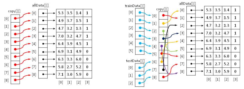
Figure 3-c: Creating Training and Test Matrices by Reference

After creating a reference copy, the next step is to scramble the order of the copy. This is shown on the right. After scrambling, the last step is to create training and test matrices by reference. In Figure 3-c, the first row of training data points to the first cell in the copy, which in turn points to the second row of the data. In other words, trainData[0][0] is 4.9, trainData[0][1] is 3.7, and so on. Similarly, testData[0][0] is 6.4, testData[0][1] is 3.9 and so on.

The definition of method MakeTrainTest begins with:

static void MakeTrainTest(double[][] allData, int seed,

      out double[][] trainData, out double[][] testData)

{

  Random rnd = new Random(seed);

  int totRows = allData.Length;

  int numTrainRows = (int)(totRows * 0.80);

  int numTestRows = totRows - numTrainRows;

. . .

The local Random object will be used to scramble row order. It accepts a seed parameter, so you can generate different results by passing in a different seed value. Here, for simplicity, the percentage split is hard-coded as 80-20. A more flexible approach is to pass the train percentage as a parameter, being careful to handle 0.80 versus 80.0 values for 80 percent.

The reference copy is made:

double[][] copy = new double[allData.Length][];

for (int i = 0; i < copy.Length; ++i)

  copy[i] = allData[i];

When working with references, even simple code can be tricky. For example, allData[0][0] is a cell value, like 4.5, but allData[0] is a reference to the first row of data.

Next, the rows of the copy matrix are scrambled, also by reference:

for (int i = 0; i < copy.Length; ++i)

{

  int r = rnd.Next(i, copy.Length);

  double[] tmp = copy[r];

  copy[r] = copy[i];

  copy[i] = tmp;

}

The scramble code uses the clever Fisher-Yates mini-algorithm. The net result is that the references in the copy matrix will be reordered randomly as suggested by the colored arrows in Figure 3-c. Method MakeTrainTest finishes by assigning the first 80% of scrambled rows in the copy matrix to the training out-matrix and the remaining rows to the test out-matrix:

. . .
  for (int i = 0; i < numTrainRows; ++i)

    trainData[i] = copy[i];

  for (int i = 0; i < numTestRows; ++i)

    testData[i] = copy[i + numTrainRows];

}

Defining the LogisticClassifier Class

The structure of the program-defined LogisticClassifier class is presented in Listing 3-b. The class has three data members. Variable numFeatures holds the number of predictor variables for a problem. Array weights holds the values used to compute outputs.

Listing 3-b: The LogisticClassifier Class

Class member rnd is a Random object that is used during the training process to generate random possible solutions.

The class exposes a single constructor and four public methods. Method Train uses a technique called simplex optimization to find values for the weights array, so that computed output values closely match the known output values in the training data.

Method ComputeOutput accepts some x-data and a set of weight values and returns a raw value between 0.0 and 1.0. This output is used by the training method to compute error. Method ComputeDependent is similar to method ComputeOutput, except that it returns a 0 or 1 result. This output is used to compute accuracy. Public method Accuracy accepts a set of weights and a matrix of either training data or test data, and returns the percentage of correct predictions.

There are five private methods: Error, RandomSolutionWts, ReflectedWts, ExpandedWts, and ContractedWts. All of these methods are used by method Train when searching for the best set of weight values.

The LogisticClassifier contains a nested private class named Solution. This class is used during training to define potential solutions, that is, potential best sets of weight values. The Solution class could have been defined outside the LogisticClassifier class, but you can define Solution as a nested class for a slightly cleaner design.

The LogisticClassifier constructor is very simple:

public LogisticClassifier(int numFeatures)

{

  this.numFeatures = numFeatures; // number predictors

  this.weights = new double[numFeatures + 1]; // [0] = b0 constant

}

If you review how the logistic regression calculation works, you'll see that the number of weight b-values has to be one more than the number of feature x-values because each x-value has an associated weight and there is one additional weight for the b₀ constant. An alternative design is to store the b₀ value in a separate variable.

Method ComputeOutput is simple, but does have one subtle point. The method is defined:

public double ComputeOutput(double[] dataItem, double[] weights)

{

  double z = 0.0;

  z += weights[0]; // b0 constant

  for (int i = 0; i < weights.Length - 1; ++i) // data might include Y

    z += (weights[i + 1] * dataItem[i]); // skip first weight

  return 1.0 / (1.0 + Math.Exp(-z));

}

For flexibility, the method accepts an array parameter named dataItem, which can represent a row of training data or test data, including a Y-value in the last cell. However, the Y-value is not used to compute output.

Method ComputeDependent is defined:

public int ComputeDependent(double[] dataItem, double[] weights)

{

  double sum = ComputeOutput(dataItem, weights);

  if (sum <= 0.5)

    return 0;

  else

    return 1;

}

Here, instead of returning a raw output value, for example 0.5678, the method returns the corresponding Y-value, which is either 0 or 1. The choice of <= instead of < is arbitrary, and has no significant effect on the operation of the classifier. A design alternative is to return a third value indicating the decision is too close to call:

if (sum <= 0.45)

  return 0;

else if (sum >= 0.45)

  return 1;
else
  return -1; // undecided

Using this alternative would require quite a few changes to the demo program code logic.

Error and Accuracy

The ultimate goal of a prediction model is accuracy, which is the percentage of correct predictions made divided by the total number of predictions made. But when searching for the best set of weight values, it is better to use a measure of error rather than accuracy. Suppose some set of weights yields these results for five training items:

Training Y   Computed Output   Computed Y   Result
--------------------------------------------------
    0            0.4980            0        correct
    1            0.5003            1        correct
    0            0.9905            1        wrong
    1            0.5009            1        correct
    0            0.4933            0        correct

The model is correct on four of the five items for an accuracy of 80%. But on the four correct predictions, the output is just barely correct, meaning output is just barely under 0.5 when giving a 0 for Y and just barely above 0.5 when giving a 1 for Y. And on the third training item, which is incorrectly predicted, the computed output of 0.9905 is not close at all to the desired output of 0.00. Now suppose a second set of weights yields these results:

Training Y   Computed Output   Computed Y   Result
--------------------------------------------------
    0            0.0008            0        correct
    1            0.9875            1        correct
    0            0.5003            1        wrong
    1            0.9909            1        correct
    0            0.5105            0        wrong

These weights are correct on three out of five for an accuracy of 60%, which is less than the 80% of the first weights, but the three correct predictions are "very correct" (computed Y is close to 0.00 or 1.00) and the two wrong predictions are just barely wrong. In short, when training, predictive accuracy is too coarse, so using error is better.

The definition of method Accuracy begins:

public double Accuracy(double[][] trainData, double[] weights)

{

  int numCorrect = 0;

  int numWrong = 0;

  int yIndex = trainData[0].Length - 1;

. . .

Counters for the number of correct and wrong predictions are initialized, and the index in a row of training data where the dependent y-value is located is specified. This is the last column. The term trainData[0]  is the first row of data, but because all rows of data are assumed to be the same, any row could have been used. Each row of data in the demo has four items, so the value of Length - 1 will be 3, which is the index of the last column. Next, the training data is examined, and its accuracy is computed and then returned:

. . .

  for (int i = 0; i < trainData.Length; ++i)

  {

    double computed = ComputeDependent(trainData[i], weights);

    double desired = trainData[i][yIndex]; // 0.0 or 1.0

    if (computed == desired)

      ++numCorrect;

    else

      ++numWrong;

  }

  return (numCorrect * 1.0) / (numWrong + numCorrect);

}

Notice that local variable computed is declared as type double, even though method ComputeDependent returns an integer 0 or 1. So an implicit conversion from 0 or 1, to 0.0 or 1.0 is performed. Therefore the condition computed == desired is comparing two values of type double for exact equality, which can be risky. However, the overhead of comparing the two values for "very-closeness" rather than exact equality is usually not worth the performance price:

double closeness = 0.00000001; // often called 'epsilon' in ML

if (Math.Abs(computed - desired) < closeness)

  ++numCorrect;

else

  ++numWrong;

The ability to control when and if to take shortcuts like this to improve performance is a major advantage of writing custom machine learning code, compared to using an existing system written by someone else where you don't have access to source code.

Method Error is very similar to method Accuracy:

private double Error(double[][] trainData, double[] weights)

{

  int yIndex = trainData[0].Length - 1;

  double sumSquaredError = 0.0;

  for (int i = 0; i < trainData.Length; ++i)

  {

    double computed = ComputeOutput(trainData[i], weights);

    double desired = trainData[i][yIndex]; // ex: 0.0 or 1.0

    sumSquaredError += (computed - desired) * (computed - desired);

  }

  return sumSquaredError / trainData.Length;

}

Method Error computes the mean squared error (sometimes called mean square error), which is abbreviated MSE in machine learning literature. Suppose there are just three training data items that yield these results:

Training Y   Computed Output
----------------------------
    0            0.3000
    1            0.8000
    0            0.1000

The sum of squared errors is:

sse = (0 - 0.3000)² + (1 - 0.8000)² + (0 - 0.1000)²
      = 0.09 + 0.04 + 0.01
      = 0.14

And the mean squared error is:

MSE = 0.14 / 3
         = 0.4667

A minor alternative is to use root mean squared error (RMSE), which is just the square root of the MSE.

Understanding Simplex Optimization

The most difficult technical challenge of any classification system is implementing the training sub-system. Recall that there are roughly a dozen major approaches with names like simple gradient descent, Newton-Raphson, back-propagation, and L-BFGS. All of these algorithms are fairly complex. The demo program uses a technique called simplex optimization.

Loosely speaking, a simplex is a triangle. The idea behind simplex optimization is to start with three possible solutions. One possible solution will be "best" (meaning smallest error), one will be "worst" (largest error), and the third is called "other". Next, simplex optimization creates three new possible solutions called "expanded", "reflected", and "contracted". Each of these is compared against the current worst solution, and if any of the new candidates is better (smaller error) than the current worst, the worst solution is replaced.

Expressed in very high-level pseudo-code, simplex optimization is:

create best, worst, other possible solutions
loop until done
  create expanded, reflected, contracted candidate replacements
  if any are better than worst, replace worst
  else if none are better, adjust worst and other solutions
end loop

Simplex optimization is illustrated in Figure 3-d. In a simple case where a solution consists of two values, like (1.23, 4.56), you can think of a solution as a point on the (x, y) plane. The left side of Figure 3-d shows how three new candidate solutions are generated from the current best, worst, and “other” solutions.

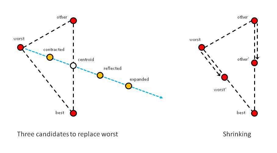
Figure 3-d: Simplex Optimization

First, a centroid is computed. The centroid is the average of the best and “other” solutions. In two dimensions, this is a point half-way between the "other" and best points. Next, an imaginary line is created, which starts at the worst point and extends through the centroid. Now, the contracted candidate is between the worst and centroid points. The reflected candidate is on the imaginary line, past the centroid. And the expanded candidate is past the reflected point.

In each iteration of simplex optimization, if one of the expanded, reflected, or contracted candidates is better than the current worst solution, worst is replaced by that candidate. If none of the three candidates generated are better than the worst solution, the current worst and "other" solutions are moved toward the best solution to points somewhere between their current position and the best solution, as shown in the right-hand side of Figure 3-d.

After each iteration, a new virtual "best-other-worst" triangle is formed, getting closer and closer to an optimal solution. If a snapshot of each triangle is taken, when looked at sequentially, the moving triangles resemble a pointy blob moving across the plane in a way that resembles a single-celled amoeba. For this reason, simplex optimization is sometimes called amoeba method optimization.

There are many variations of simplex optimization, which vary in how far the contracted, reflected, and expanded candidate solutions are from the current centroid, and the order in which the candidate solutions are checked to see if each is better than the current worst solution. The most common variation of simplex optimization is called the Nelder-Mead algorithm. The demo program uses a simpler variation that does not have a specific name.

In pseudo-code, the variation of simplex optimization used in the demo program is:

randomly initialize best, worst, other solutions
loop maxEpochs times
  create centroid from worst and other
  create expanded
  if expanded is better than worst, replace worst with expanded,
    continue loop
  create reflected
  if reflected is better than worst, replace worst with reflected,
    continue loop
  create contracted
  if contracted is better than worst, replace worst with contracted,
    continue loop
  create a random solution
  if  random solution is better than worst, replace worst,
    continue loop
  shrink worst and other toward best
end loop
return best solution found

Simplex optimization, like all other machine learning optimization algorithms, has pros and cons. This is why there are so many different optimization techniques, each with dozens of variations. In real-life scenarios, somewhat surprisingly, no machine learning optimization technique guarantees you will find the optimal solution, if one exists. However, simplex optimization is relatively simple to implement and usually, but not always, works well in practice.

Training

The goal of the logistic regression classifier training process is to find a set of weight values so that when presented with training data, the computed output values closely match the known output values. In other words, the goal of training is to minimize the error between computed output values and known output values. This is called a numerical optimization problem because you want to optimize weight values to minimize error.

Class method Train uses a local class named Solution as part of the simplex optimization. A solution represents a possible solution to the problem of finding the weight values that minimize error. A Solution object is a collection of weights and the mean squared error associated with those weights. The definition is presented in Listing 3-c.

Listing 3-c: The Solution Helper Class Definition

The key concept of simplex optimization is that there is a best, worst, and "other" solution, so the three current solutions must be sorted by error, from smallest error to largest. Notice that helper class Solution derives from the IComparable interface. What his means is that a collection of Solution objects can be sorted automatically.

Using a private nested class that derives from the IComparable interface is a rather exotic approach. When programming, simple is almost always better than exotic and clever (in my opinion, anyway), but in this situation, the simplification of the code in the Train method is worth the overhead of a not-very-straightforward programming technique.

The definition of method Train begins with:

public double[] Train(double[][] trainData, int maxEpochs, int seed)

{

  this.rnd = new Random(seed);

  Solution[] solutions = new Solution[3]; // best, worst, other

  for (int i = 0; i < 3; ++i)

  {

    solutions[i] = new Solution(numFeatures);

    solutions[i].weights = RandomSolutionWts();

    solutions[i].error = Error(trainData, solutions[i].weights);

  }
. . .

First, the class member Random object rnd is instantiated with a seed value. This instantiation is performed inside method Train rather than in the constructor, so that if you wanted, you could restart training several times, using a different seed value each time to get different results.

Next, an array of Solution objects is instantiated. The whole point of going to the trouble of creating a Solution object is so that an array of solutions can be sorted to give the best, worst, and "other". The Solution object in each cell of the solutions array is instantiated by calling the constructor, and then a helper method named RandomSolutionWts supplies the values for the weights, and method Error supplies the mean squared error.

Next, the main training loop is created:

int best = 0;

int other = 1;

int worst = 2;

int epoch = 0;

while (epoch < maxEpochs)

{

  ++epoch;
. . .

Local variables best, other, and worst are set up for clarity. For example, the expression

solutions[2].weights[0]

is the first weight value in the worst solution because Solution objects are ordered from smallest error to largest. Using the local variable instead, the expression would be:

solutions[worst].weights[0]

This is a bit more clear, and likely less error-prone. The local variable epoch is just a loop counter. Inside the main loop, the three possible solutions are sorted and the centroid is computed:

Array.Sort(solutions);

double[] bestWts = solutions[0].weights; // convenience only

double[] otherWts = solutions[1].weights;

double[] worstWts = solutions[2].weights;

double[] centroidWts = CentroidWts(otherWts, bestWts);

This is where the private Solution class shows its worth, by allowing the array of Solution objects to be sorted automatically, from smallest error to largest, simply by calling the built-in Array.Sort method. As before, for convenience and clarity, the weights arrays of the three Solution objects receive local aliases bestWts, otherWts, and worstWts. Helper method CentroidWts computes a centroid based on the weights in the current best and "other" solutions.

Next, the expanded candidate replacement for the current worst solution is created. If the expanded candidate is better than the worst solution, the worst solution is replaced:

double[] expandedWts = ExpandedWts(centroidWts, worstWts);

double expandedError = Error(trainData, expandedWts);

if (expandedError < solutions[worst].error)

{

  Array.Copy(expandedWts, worstWts, numFeatures + 1);

  solutions[worst].error = expandedError;

  continue;

}

Replacing the current worst solution requires two steps. First, the weights have to be copied from the candidate into worst, and then the error term has to be copied in. This is allowed because Solution class members weights and error were declared with public scope.

As a very general rule of thumb, using the continue statement inside a while-loop can be a bit tricky, because many statements in the loop after the continue statement are skipped. In this situation, however, using the continue statement leads to cleaner and more easily modified code than the alternative of a deeply nested if-else-if structure.

If the expanded candidate is not better than the worst solution, the reflected candidate is created and examined:

double[] reflectedWts = ReflectedWts(centroidWts, worstWts);

double reflectedError = Error(trainData, reflectedWts);

if (reflectedError < solutions[worst].error)

{

  Array.Copy(reflectedWts, worstWts, numFeatures + 1);

  solutions[worst].error = reflectedError;

  continue;

}

If the reflected candidate is not better than the worst solution, the contracted candidate is created and examined:

double[] contractedWts = ContractedWts(centroidWts, worstWts);

double contractedError = Error(trainData, contractedWts);

if (contractedError < solutions[worst].error)

{

  Array.Copy(contractedWts, worstWts, numFeatures + 1);

  solutions[worst].error = contractedError;

  continue;

}

At this point, none of the three primary candidate solutions are better than the worst solution, so a random solution is tried:

double[] randomSolWts = RandomSolutionWts();

double randomSolError = Error(trainData, randomSolWts);

if (randomSolError < solutions[worst].error)

{

  Array.Copy(randomSolWts, worstWts, numFeatures + 1);

  solutions[worst].error = randomSolError;

  continue;

}

Generating a candidate solution and computing its associated mean squared error is a relatively expensive operation because every training data item must be processed. So an alternative to consider is to attempt a random solution every so often, say, just once for every 100 iterations:

if (epoch % 100 == 0)

{

  // create and examine a random solution

} 

Now at this point, no viable replacement for the worst solution was found, so the simplex shrinks in on itself by moving the worst and "other" solutions toward the best solution:

. . .

  for (int j = 0; j < numFeatures + 1; ++j)

    worstWts[j] = (worstWts[j] + bestWts[j]) / 2.0;

  solutions[worst].error = Error(trainData, solutions[worst].weights);

  for (int j = 0; j < numFeatures + 1; ++j)

    otherWts[j] = (otherWts[j] + bestWts[j]) / 2.0;

  solutions[other].error = Error(trainData, otherWts);

} // while

Here, the current worst and "other" solutions move halfway toward the best solution, as indicated by the 2.0 constants in the code. The definition of method Train concludes with:

. . .

  Array.Copy(solutions[best].weights, this.weights, this.numFeatures + 1);

  return this.weights;

}

The weights in the best Solution object are copied into class member array weights. A reference to the class member weights is returned so that the best weights can be used by other methods, such as ComputeDependent in particular, to make predictions on new, previously unseen data. An alternative to returning the best weights by reference is to make a new array, copy the values from the best solution into that array, and return by value.

Helper method CentroidWts computes the centroid used by simplex optimization. Recall the centroid is an average of the current best and "other" solutions:

private double[] CentroidWts(double[] otherWts, double[] bestWts)

{

  double[] result = new double[this.numFeatures + 1];

  for (int i = 0; i < result.Length; ++i)

    result[i] = (otherWts[i] + bestWts[i]) / 2.0;

  return result;

}

Helper method ExpandedWts is defined:

private double[] ExpandedWts(double[] centroidWts, double[] worstWts)

{

  double gamma = 2.0;

  double[] result = new double[this.numFeatures + 1];

  for (int i = 0; i < result.Length; ++i)

    result[i] = centroidWts[i] + (gamma * (centroidWts[i] - worstWts[i]));

  return result;

}

Here, local variable gamma controls how far the expanded candidate is from the centroid. Larger values of gamma tend to produce larger changes in the solutions in the beginning of processing at the expense of unneeded calculations later in the processing. Smaller values of gamma tend to produce smaller changes initially, but fewer calculations later.

Helper methods ReflectedWts and ContractedWts use the exact same pattern as method ExpandedWts:

private double[] ReflectedWts(double[] centroidWts, double[] worstWts)

{

  double alpha = 1.0;

  double[] result = new double[this.numFeatures + 1];

  for (int i = 0; i < result.Length; ++i)

    result[i] = centroidWts[i] + (alpha * (centroidWts[i] - worstWts[i]));

  return result;

}

private double[] ContractedWts(double[] centroidWts, double[] worstWts)

{

  double rho = -0.5;

  double[] result = new double[this.numFeatures + 1];

  for (int i = 0; i < result.Length; ++i)

    result[i] = centroidWts[i] + (rho * (centroidWts[i] - worstWts[i]));

  return result;

}

In method ReflectedWts, with an alpha value of 1.0, multiplying by alpha obviously has no effect, so in a production scenario you could just eliminate alpha altogether. There are several ways to improve the efficiency of these three helper methods, though at the minor expense of some loss of clarity. For example, notice that each method computes the quantity centroidWts[i] - worstWts[i]. This common value could be computed just once and then passed to each method along the lines of:

for (int i = 0; i < numFeatures + 1; ++i)
  delta[i] = centroidWts[i] - worstWts[i];

double[] expandedWts = ExpandedWts(delta);
. . .
double[] reflectedWts = ReflectedWts(delta);
// etc.

Helper method RandomSolutionWts is used to initialize the three current solutions (best, worst, other), and is also used, optionally, to probe when no replacement candidate (expanded, reflected, contracted) is better than the current worst solution. The method is defined:

private double[] RandomSolutionWts()

{

  double[] result = new double[this.numFeatures + 1];

  double lo = -10.0;

  double hi = 10.0;

  for (int i = 0; i < result.Length; ++i)

    result[i] = (hi - lo) * rnd.NextDouble() + lo;

  return result;

}

The method returns an array of weights where each value is a random number between -10.0 and +10.0, for example { 3.33, -0.17, 7.92, -5.05 }. Because it is assumed that all input x-values have been normalized, the majority of x-values will be between -10.0 and +10.0, so this range is also used for the weight values. Because these two values are hard-coded, in method RandomSolutionWts you could replace term (hi - lo) with the constant 20.0, and replace variable lo with -10.0. If your x-values are not normalized, it is quite possible that constraining weight values to the interval [-10.0, +10.0] could lead to a poor model when the magnitudes of different features vary greatly.

The Train method iterates a fixed number of times specified by the maxEpochs variable:

int epoch = 0;

while (epoch < maxEpochs)

{

  ++epoch;
  // search for best weights
}

An important, recurring theme in most machine learning training algorithms is that there are many ways to control when the main training loop terminates. For simplex optimization, there are two important options to consider. First, you may want to exit early if the Euclidean distance (difference) between the current best and worst solutions reaches some very low value indicating the simplex has collapsed on itself. Second, you may want to exit only when the mean squared error drops below some acceptable level, indicating your model is likely good enough.

Other Scenarios

This chapter explains binary logistic regression classification, where the dependent variable can take one of just two possible values. There are several techniques you can use to extend logistic regression to situations where the dependent variable can take one of three or more values, for example, predicting a person's political affiliation of Democrat, Republican, or Independent. The simplest approach is called one-versus-all. You would run logistic regression for Democrat versus "others”, run a second time with Republican versus "others", and run a third time with Independent versus "others". That said, logistic regression classification is most often used for binary problems.

Logistic regression classification can handle problems where the predictor variables are numeric, such as the kidney score feature in the demo program, or categorical, such as the sex feature in the demo. For a categorical x-variable with two possible values, such as sex, the values are encoded as -1 or +1. For x-variables that have three or more possible values, the trick is to use a technique called 1-of-(N-1) encoding. For example, if three predictor values are "small","medium", and "large", the values would be encoded as (1, 0), (0, 1), and (-1, -1), respectively.

Chapter 3 Complete Demo Program Source Code