Multiclass Classification

The goal of multiclass classification is to make a prediction where the variable to predict can take on one of a set of three or more discrete values. For example, you might want to predict the political party affiliation of a person (democrat, republican, or other) based on their age, sex, annual income, and so on.

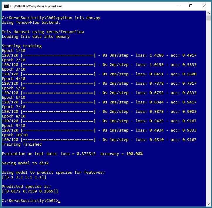
Figure 2-1: Multiclass Classification using Keras

The screenshot in Figure 2-1 shows a demonstration of multiclass classification. The demo program begins by loading 120 training data items and 30 test data items into memory. Each item represents an iris flower where the four predictor variables are sepal length, sepal width, petal length, and petal width (a sepal is a leaf-like structure). The variable to predict is species. There are three possible species: setosa, versicolor, and virginica.

Behind the scenes, the demo program creates a 4-(5-6)-3 neural network, that is, one with four input values (one for each predictor variable), two hidden layers with five and six nodes respectively, and three output nodes (one for each possible species). The demo program trains the neural network model using 10 epochs.

After training completes, the trained model achieves a prediction accuracy of 100.00% on the test data (30 of 30 correct). The demo concludes by making a prediction for a new, previously unseen iris flower with predictor values (6.1, 3.1, 5.1, 1.1). The predicted probabilities are (0.0172, 0.7159, 0.2669), and because the second value is largest, the prediction is versicolor.

Understanding the data

Fischer's Iris dataset is one of the most well-known benchmark datasets in statistics and machine learning. There are a total of 150 items. The raw data looks like:

5.1, 3.5, 1.4, 0.2, setosa
7.0, 3.2, 4.7, 1.4, versicolor
6.3, 3.3, 6.0, 2.5, virginica

The raw data was prepared by one-hot encoding the class labels, but the feature values were not normalized as is usually done:

5.1, 3.5, 1.4, 0.2, 1, 0, 0
7.0, 3.2, 4.7, 1.4, 0, 1, 0
6.3, 3.3, 6.0, 2.5, 0, 0, 1

After encoding, the full dataset was split into a 120-item set for training, and a 30-item test set to be used after training for model evaluation. Because the data has four dimensions, it's not possible to easily visualize it in a two-dimensional graph, but you can get a rough idea of the data from the partial graph in Figure 2-2.  

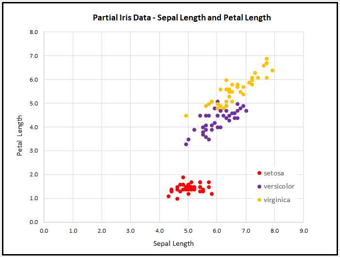
Figure 2-2: Iris Data

As the graph shows, the Iris Dataset is almost too simple. The class setosa can be easily distinguished from versicolor and virginica. Furthermore, the classes versicolor and virginica are nearly linearly separable. However, the Iris Dataset serves well as a simple example.

By the way, there are actually at least two different versions of Fisher's Iris Data that are in common use. The original data was collected in 1935, and then published by Fisher in 1936. However, at some point in time, a couple of the original values for setosa items were incorrectly copied, and years later made their way onto the Internet. This isn't serious, since the datasets are now used just for a teaching example, rather than for serious research.

The Iris program

The complete program that generated the output shown in Figure 2-1 is shown in Code Listing 2-1. The program begins with comments for the program file name and the versions of Python, TensorFlow and Keras used, and then imports the NumPy, Keras, TensorFlow, and OS packages:

# iris_dnn.py
# Python 3.5.2, TensorFlow 2.1.5, Keras 1.7.0
import numpy as np
import keras as K
import tensorflow as tf
import os
os.environ['TF_CPP_MIN_LOG_LEVEL']='2'

In a non-demo scenario, you'd want to include additional details in the comments. Because Keras and TensorFlow are under rapid development, you should always document which versions are being used. Version incompatibilities can be a significant problem when working with Keras and other open-source software.

Code Listing 2-1: Iris Multiclass Classification Program

The program imports the entire Keras package and assigns an alias K. An alternative approach is to import only the modules you need, for example:

from keras.models import Sequential
from keras.layers import Dense, Activation

Even though Keras uses TensorFlow as its backend engine, you don't need to explicitly import TensorFlow, except to set its random seed. The OS package is imported only so that an annoying TensorFlow startup warning message will be suppressed.

The program structure consists of a single main function, with no helper functions. The program begins with:

def main():
  # 0. get started
  print("\nIris dataset using Keras/TensorFlow ")
  np.random.seed(4)
  tf.set_random_seed(13)

  # 1. load data
  print("Loading Iris data into memory \n")
  train_file = ".\\Data\\iris_train.txt"
  test_file = ".\\Data\\iris_test.txt"
. . .

In most situations, you want to make your results reproducible. The Keras library makes extensive use of the NumPy global random number generator, so it's good practice to set the seed value. The value used in the program, 4, is arbitrary. Similarly, because Keras uses TensorFlow, you'll usually want to set its seed, too. However, program results typically aren't completely reproducible due to order of numeric rounding of parallelized tasks.

I indent with two spaces rather than the normal four spaces because of page-width limitations. All normal error-checking has been removed to keep the main ideas as clear as possible.

The program assumes that the training and test data files are located in a subdirectory named Data. The program doesn't have any information about the structure of the data files. I strongly recommend that you include program comments such as:

# data is comma-delimited and looks like:
# 5.1, 3.5, 1.4, 0.2, 1, 0, 0
# first four values are non-normalized features
# last three values are one-hot labels for
# setosa, versicolor, virginica
# 120 training items, 30 test items

This kind of information is easy to remember when you're writing your program, but difficult to remember a couple of weeks later.

The training and test data are read into memory with these statements:

  train_x = np.loadtxt(train_file, usecols=[0,1,2,3],
   delimiter=",",  skiprows=0, dtype=np.float32)
  train_y = np.loadtxt(train_file, usecols=[4,5,6],
    delimiter=",", skiprows=0, dtype=np.float32)

  test_x = np.loadtxt(test_file, usecols=range(0,4),
   delimiter=",",  skiprows=0, dtype=np.float32)
  test_y = np.loadtxt(test_file, usecols=range(4,7),
    delimiter=",", skiprows=0, dtype=np.float32)

In general, Keras needs feature data and label data stored in separate NumPy array-of-array style matrices. There are many ways to read data into memory, but the loadtxt() function is versatile enough to meet most problem scenarios. The NumPy genfromtxt() function is very similar but gives you a few additional options, such as dealing with missing data. The loadtxt() function has a large number of parameters, but in most cases, you only need usecols, delimiter, and dtype. 

Notice that usecols can accept a list such as [0,1,2,3] or a Python range such as range(0,4). If you use the range() function, be careful to remember that the first parameter is inclusive, but the second parameter is exclusive.

In addition to the comma character, common values for the delimiter parameter are "\t" (tab) and " " (single space) The default parameter value is None, which means any whitespace.

The default dtype parameter value is numpy.float, which is an alias for Python float, and is the exact same as numpy.float64. But the default data type for almost all Keras functions is numpy.float32, so the program specifies this type. The idea is that for the majority of machine-learning problems, the advantage in precision gained by using 64-bit values is not worth the memory and performance penalty.

An alternative approach to using static, separate training and test files is to use just a single file containing all data, read all data into memory, and then programmatically generate training and test matrices in memory. This alternative technique allows you to perform k-fold cross validation, a technique which used to be common, but which is now rarely used with deep learning and very large datasets.

Instead of using a NumPy function such as loadtxt() to read data into memory, a different approach is to use the Pandas (originally "panel data," now "Python Data Analysis Library") library, which has many advanced data manipulation features. However, Pandas has a significant learning curve.

Defining the neural network model

The program defines a 4-(5-6)-3 deep neural network using this code:

  # 2. define model
  init = K.initializers.glorot_uniform(seed=1)
  simple_adam = K.optimizers.adam()
  model = K.models.Sequential()
  model.add(K.layers.Dense(units=5, input_dim=4, kernel_initializer=init,
    activation='relu'))
  model.add(K.layers.Dense(units=6, kernel_initializer=init,
    activation='relu'))
  model.add(K.layers.Dense(units=3, kernel_initializer=init,
    activation='softmax'))

  model.compile(loss='categorical_crossentropy',
    optimizer=simple_adam, metrics=['accuracy'])

Deep neural networks are often very sensitive to the initial values of the weights and biases, so Keras has several different initialization functions. The demo uses glorot_uniform(), which assigns small, random values based on the fan-in and fan-out of the network layer in which it's used. The seed parameter is used so that program results will be reproducible. Table 2-1 lists a few of the common initialization functions in Keras.

Table 2-1: Common keras.initializers Functions

The program prepares an Adam() optimizer object to be used by the fit() training function. Adam (adaptive moment estimation) is one of many training algorithms supported by Keras, and it's a good first choice when creating a prediction model. The program uses all Adam() default parameters, but they could have been specified explicitly as a form of documentation:

simple_adam = K.optimizers.Adam(lr=0.001, beta_1=0.9, beta_2=0.999,
  epsilon=None, decay=0.0, amsgrad=False) # default parameter values

The program builds up the neural network architecture using the Sequential() method. The input layer is implicit, so the model begins with the first hidden layer:

  model = K.models.Sequential()
  model.add(K.layers.Dense(units=5, input_dim=4, kernel_initializer=init,
    activation='relu'))

The Dense() function is a standard, fully-connected layer. The units parameter specifies the number of hidden processing nodes in the layer, and because this is the first layer listed, you must specify how many input values there are using the input_dim parameter.

The hidden layer is configured to use relu activation (rectified linear unit). As you might expect, Keras supports many activation functions. For a Dense() hidden layer, relu is often a good first attempt. Other common activation functions are listed in Table 2-2. Keras also contains advanced, adaptive activation functions such LeakyReLU() in the keras.layers module.

Table 2-2: Common Dense Layer Activation Functions

An alternative to supplying a string value like 'relu' to the activation parameter of the Dense() function, which uses default parameter values in the case of relu() and softmax(), is to use an Activation layer. For example:

  model = K.models.Sequential()
  model.add(K.layers.Dense(units=5, input_dim=4, kernel_initializer=init))
  model.add(K.layers.Activation('relu'))

One of the challenges of working with Keras is that as it has evolved over time, many different techniques have been created, which can be confusing. Sometimes older examples use one approach, such as a separate Activation layer, and newer examples use a different approach, such as the string activation parameter in Dense().

After setting up the implied input layer and the explicit first hidden layer, the rest of the architecture is specified like so:

  model.add(K.layers.Dense(units=6, kernel_initializer=init,
    activation='relu'))
  model.add(K.layers.Dense(units=3, kernel_initializer=init,
    activation='softmax'))

Because neither of these are the first layer, you don't have to specify the number of input values. If you wanted to, you could do so like this:

  model.add(K.layers.Dense(units=6, input_dim=5, kernel_initializer=init,
    activation='relu'))
  model.add(K.layers.Dense(units=3, input_dim=6, kernel_initializer=init,
   activation='softmax'))

Instead of using Sequential() and the add() method, you can construct a neural network by creating separate layers and then passing them to the Model() constructor like this:

  init = K.initializers.glorot_uniform(seed=1)
  X = K.layers.Input(shape=(4,))
  net = K.layers.Dense(units=5, kernel_initializer=init,
    activation='relu')(X)
  net = K.layers.Dense(units=6, kernel_initializer=init,
    activation='relu')(net)
  net = K.layers.Dense(units=3, kernel_initializer=init,
    activation='softmax')(net)
  model = K.models.Model(X, net)

The two approaches create the exact same neural network, but are quite different in terms of syntax. For multiclass classification problems, the choice is purely one of personal preference.

After a neural network model has been defined, it must be compiled before it can be trained:

  model.compile(loss='categorical_crossentropy',
    optimizer=simple_adam, metrics=['accuracy'])

You can loosely think of the compilation process as translating Keras code into TensorFlow code (or CNTK code or Theano code). You must pass values to the optimizer and loss parameters so that the fit() method will know how to train the model. For multiclass classification, the categorical_crossentropy loss function is usually the best choice, but you can use the mean_squared_error function if needed (for example, to replicate the work of other people).

The metrics parameter is optional. The program passes a Python list containing just 'accuracy' to indicate that classification accuracy (percentage correct predictions) should be computed during training.

Training and evaluating the model

After training data has been read into memory and the neural network has been created, the program trains the model using these statements:

  # 3. train model
  b_size = 1
  max_epochs = 10
  print("Starting training ")
  h = model.fit(train_x, train_y, batch_size=b_size, epochs=max_epochs,
    shuffle=True, verbose=1)
  print("Training finished \n")

The batch size is set to 1, which is called online training. This means that the neural network weights and biases are updated for every training item. Alternatives are to set the batch size to the number of items in the training set (120), which is sometimes called full-batch training, or to set the batch size to an intermediate value such as 16, which is called mini-batch training.

The max_epochs variable controls how many iterations will be used for training. The shuffle parameter in the fit() function indicates that the training items should be processed in random order. The default value is True, so the parameter could have been omitted. The verbose parameter controls how much information to display during training: 0 means display no information, 1 means display full information, and 2 means display a medium amount of information.

The fit() function returns a dictionary object that has the recorded training history. The demo program captures this information into object h, but doesn't make use of it. If you wanted to see the loss values, you could do so like this:

print(h.history['loss']) 

After training, the demo program evaluates the model on the test data:

  # 4. evaluate model
  eval = model.evaluate(test_x, test_y, verbose=0)
  print("Evaluation on test data: loss = %0.6f  accuracy = %0.2f%% \n" \
    % (eval[0], eval[1]*100) )

The evaluate() function returns a list of values. The first value at index [0] is the always value of the required loss function specified in the compile() function. Other values in the list are any optional metrics from the compile() function. In this example, 'accuracy' was passed, so the value at index [1] holds the classification accuracy. The program multiples by 100 to convert accuracy from a proportion (like 0.9123) to a percentage (like 91.23%).

Saving and using the model

In most situations you'll want to save a trained model, especially if the training took hours or even longer. The demo program saves the trained model like so:

  # 5. save model
  print("Saving model to disk \n")
  mp = ".\\Models\\iris_model.h5"
  model.save(mp)

Somewhat unusually, compared to other neural network libraries, Keras saves a trained model using the hierarchical data format (HDF) version 5. It is a binary format, so saved models can't be inspected with a text editor. In addition to saving an entire model, you can save just the model weights and biases, which is sometimes useful. You can also save the just model architecture but not the weights.

A saved Keras model can be loaded from a different program like this:

print("Loading a saved model")
mp = ".\\Models\\iris_model.h5"
model = K.models.load_model(mp)

The whole point of creating and training a model is so that it can be used to make predictions for new, previously unseen data:

   # 6. use model
  np.set_printoptions(precision=4)
  unknown = np.array([[6.1, 3.1, 5.1, 1.1]], dtype=np.float32)
  predicted = model.predict(unknown)
  print("Using model to predict species for features: ")
  print(unknown)
  print("\nPredicted species is: ")
  print(predicted)

The predict() method accepts input and computes output based on the values of the model's current weights and biases. Notice that variable unknown is an array-of-arrays (indicated by the double square brackets) rather than a simple vector.

The output is raw in the sense that it's a set of probabilities. It's up to you to interpret the meaning. You can do so programmatically along the lines of:

  labels = ["setosa", "versicolor", "virginica"]
  idx = np.argmax(predicted)
  species = labels[idx]
  print(species)

The argmax(v) function returns the index of the largest value in vector or list v. It's a useful function for many classification problems.

Summary and resources

To perform multiclass classification, you encode the target labels using one-hot (also called 1-of-N) encoding. The activation function on the output layer should be set to softmax so the node values sum to 1.0, and can be loosely interpreted as probabilities.

The loss function in most cases should be set to categorical_crossentropy, but you can use mean_squared_error if you wish. In general, you should pass accuracy to the optional metrics list of the compile() function.

Free parameters for multiclass classification include the number of hidden layers and the number of nodes in each hidden layer, the optimizer algorithm (but Adam is often a good choice), batch size, and the maximum number of training epochs to use.

The training and test data used by the demo program can be found here.

The demo program uses the glorot_uniform() function for initialization. See additional information and alternatives here.

The demo program uses the relu() function for hidden-layer activation. See additional information and alternatives here.