Image Classification

The goal of image classification is to make a prediction where the variable to predict is a label that's associated with an image. For example, you might want to predict whether a photograph contains an "apple," "banana," or "orange." The most common way to perform image classification is to use what's called a convolutional neural network (CNN).

Figure 5-1: Image Classification on the MNIST Dataset Using Keras

The screenshot in Figure 5-1 shows a demonstration of image classification. The demo program begins by loading 1,000 training images and 100 test images into memory. Each image is a handwritten digit from '0' to '9' and is 28 pixels wide by 28 pixels tall, for a total of 784 pixels. The data is a subset of the MNIST (modified National Institute of Standards and Technology) benchmark dataset.

Behind the scenes, the demo program creates a 784-32-64-100-10 convolutional neural network. The network has 784 input nodes and 10 output nodes, one for each possible digit or label. The meaning of the 32-64-100 part of the architecture will be explained shortly. The demo program trains the neural network model using 50 epochs. During training, the loss and accuracy values for the training data are displayed to make sure that training is making progress.

After training completes, the trained model achieves a prediction accuracy of 98.00 percent on the test data (98 of 100 images correct, 2 incorrect). The demo concludes by making a prediction for a dummy, hypothetical, previously unseen image that vaguely resembles a handwritten digit. The predicted digit is a '6' because the largest value (1.0) of the output probabilities vector is at index [6].

Understanding the data

The MNIST dataset is essentially the "Hello World" dataset for deep learning. The full dataset consists of 60,000 training images and 10,000 test images. The demo program uses a subset of MNIST (1,000 training images and 100 test images) for simplicity.

Each of the 28x28 pixels is a grayscale integer value between 0 (white) and 255 (black). Figure 5-2 shows the first training image, displayed as 784 pixel values in hexadecimal format, and also as an image.

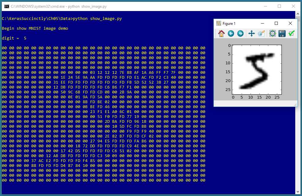
Figure 5-2: A Typical MNIST Image

The raw data is stored in an unusual format, and before coding the demo program, the raw data has to be preprocessed. Both the raw training and raw test datasets are stored in two files each. The first file contains just the pixel values, 784 values per line (60,000 lines for the training file, 10,000 lines for the test file). The second file contains just the labels, '0' through '9', one per line.

Additionally, all four files are stored in a proprietary binary format, and in big endian format, rather than in the far more common little endian format used by Intel and similar processors. And the four source files are compressed in .gz format.

First, the four raw source files are unzipped. For the training data, the preprocessing in high level pseudo-code is:

open (binary) pixel file for reading
open (binary) labels file for reading
open (text) result file for writing

read and discard header bytes in pixels and labels file

loop 1000 times
  read label from label file
  write label to result file
  write "##" separator
  loop 784 times
    read a pixel byte
    write pixel to result file
  end-loop
  write a newline to result file
end-loop
close all files

The result is a training file with 1000 lines that looks like this:

2 ** 0 0 152 27 .. 0
5 ** 0 0 38 122 .. 0

The first value is the lass label, '0' through '9'. Next is a double-asterisk separator, just for readability. Next are the 784 pixel values. The 100-image test file has the same structure. The preprocessing does not encode the class labels, and does not normalize the pixel values. As you'll see shortly, encoding and normalization are done programmatically.

When working with machine learning, getting your data ready is often time-consuming, annoying, and difficult. It's not uncommon for data preprocessing to require 90 percent (or more) of your total time and effort.

Note that the Keras library comes with a pre-processed MNIST dataset that can be accessed like this:

from keras.datasets import mnist
(train_x, train_y), (test_x, test_y) = mnist.load_data()

However, this is a bit of a cheat because in a non-demo scenario, you won't have a nice way like this to access your data.

The MNIST program

The complete program that generated the output shown in Figure 5-1 is shown in Code Listing 5-1. The program begins with comments for the program file name (the _cnn is not a standard convention, and just stands for convolutional neural network) and versions of Python, TensorFlow, and Keras used, and then imports the NumPy, Keras, TensorFlow, and OS packages. The PyPlot module is also imported so that the dummy input image can be displayed:

# mnist_cnn.py
# Python 3.5.2, TensorFlow 2.1.5, Keras 1.7.0
import numpy as np
import keras as K
import tensorflow as tf
import os
os.environ['TF_CPP_MIN_LOG_LEVEL']='2'
import matplotlib.pyplot as plt

In a non-demo scenario, you'd want to include lots of additional details in the comments. Because Keras and TensorFlow are under rapid development, it's a good idea to document which versions are being used. Version incompatibilities can be a significant problem when working with Keras and open-source software.

Code Listing 5-1: MNIST Image Classification Program

The program imports the entire Keras package and assigns an alias K. An alternative approach is to import only the modules you need, for example:

from keras.models import Sequential
from keras.layers import Dense, Activation

Even though Keras uses TensorFlow as its backend engine, you don't need to explicitly import TensorFlow, except in order to set its random seed. Instead of importing the entire TensorFlow package, you could import only the module need to set the random seed. The OS package is imported only so that an annoying TensorFlow startup warning message will be suppressed.

The program structure consists of a single main function, plus a program-defined helper class, MyLogger, for custom logging, and a program-defined helper function to programmatically encode the labels. The logging class definition is:

class MyLogger(K.callbacks.Callback):
  def __init__(self, n):
    self.n = n

  def on_epoch_end(self, epoch, logs={}):
    if epoch % self.n == 0:
      t_loss = logs.get('loss')
      t_accu = logs.get('acc')
      print("epoch = %4d  loss = %0.4f  accuracy = %0.2f%%" % \
(epoch, t_loss, t_accu*100))

The MyLogger class is used only to display loss and accuracy metrics that are computed automatically, so the class initializer doesn't need to accept references to the training data. Most program-defined callbacks would pass that information like this:

def __init__(self, n, data_x, data_y):
  self.n = n
  self.data_x = data_x
  self.data_y = data_y

The on_epoch_end() method pulls the current loss and accuracy metrics from the built-in logs dictionary and displays them. The demo program does this only so that the logging display messages can be reduced to once every 10 epochs instead of every epoch. Keras computes loss and accuracy for every training batch and averages the values over all batches at the end of each epoch. If you want more granular information, you can use the on_batch_end() method.

The main() function begins with:

def main():
  # 0. get started
  print("\nMNIST CNN demo using Keras/TensorFlow ")
  np.random.seed(1)
  tf.set_random_seed(2)

  # 1. load data
  print("Loading subset of MNIST data into memory \n")
  train_file = ".\\Data\\mnist_train_keras_1000.txt"
  test_file = ".\\Data\\mnist_test_keras_100.txt"
. . .

In most situations, you want your results to be reproducible. The Keras library uses the NumPy and TensorFlow global random-number generators, so it's good practice to set the seed values. The values used in the program, 1 and 2, are arbitrary. However, be aware that the Keras program results typically aren't completely reproducible due, in part, to order of numeric rounding of parallelized tasks.

The program assumes that the training and test data files are located in a subdirectory named Data. The demo program doesn't have any information about the structure of the data files. I recommend that you include comments in your program that explain things such as how many predictor variables there are, types of encoding and normalization used, and so on. This kind of information is easy to remember when your writing your program, but difficult to remember a couple of weeks later.

The training data is read into memory by these two statements:

  train_x = np.loadtxt(train_file, usecols=range(2,786),
    delimiter=" ", skiprows=0, dtype=np.float32)
  train_y = np.loadtxt(train_file, usecols=[0],
    delimiter=" ", skiprows=0, dtype=np.float32)

In general, Keras needs feature data and label data stored in separate NumPy array-of-array style matrices. There are many ways to read data into memory, but the loadtxt() function is versatile enough to meet most problem scenarios. An alternative approach is to use the read_csv() function from the Pandas (Python Data Analysis Library) package.

The default dtype parameter value is numpy.float, which is an alias for Python float, and is the exact same as numpy.float64. But the default data type for almost all Keras functions is numpy.float32, so the program specifies this type. The idea is that for the majority of machine learning problems, the advantage in precision gained by using 64-bit values is not worth the memory and performance penalty.

After the training data is in memory, it is encoded and normalized like so:

  train_x = train_x.reshape(train_x.shape[0], 28, 28, 1)
  train_x /= 255
  train_y = encode_y(train_y, 10)  # one-hot

A Keras CNN expects image input data as a NumPy array with four dimensions: number of items, width of image, height of image, and number of channels (1 for grayscale, 3 for an RGB image).

Because all pixel values are between 0 and 255, dividing by 255 results in all pixel values being normalized to 0.0 to 1.0, which is in effect min-max normalization. The y-values are one-hot encoded, for example, the first training image label is a '5' digit, so it is encoded as (0, 0, 0, 0, 0, 1, 0, 0, 0, 0).

The test data is read, reshaped, normalized, and encoded in the same way as the training data. The two main advantages of programmatically encoding and normalizing data are that you can easily experiment with different approaches, and that when you use the trained model to make predictions, you can use raw, unnormalized or encoded input values. The main disadvantage of programmatically encoding and normalizing is that it adds complexity to your program.

Defining the Convolutional Neural Network model

The demo program prepares to create the CNN model with these statements:

  init = K.initializers.glorot_uniform()
  simple_adadelta = K.optimizers.Adadelta()

The demo sets up initial weights using the Glorot uniform algorithm, which, because it is the default, could have been omitted. Deep neural networks are often very sensitive to the initial values of the weights and biases, so Keras has several different initialization functions you can use.

The training optimizer object is Adadelta() ("adaptive delta"), one of many advanced variations of basic stochastic gradient descent. Reasonable alternatives include RMSprop(), Adagrad(), and Adam(); however, SGD() typically does not work well for CNN image classification.

The CNN network is defined like so:

  model = K.models.Sequential()
  model.add(K.layers.Conv2D(filters=32, kernel_size=(3, 3), strides=(1,1),
    padding='same', kernel_initializer=init, activation='relu',
    input_shape=(28,28,1)))
  model.add(K.layers.Conv2D(filters=64, kernel_size=(3, 3), strides=(1,1),
    padding='same', kernel_initializer=init, activation='relu'))
  model.add(K.layers.MaxPooling2D(pool_size=(2, 2)))
  model.add(K.layers.Dropout(0.25))
  model.add(K.layers.Flatten())
  model.add(K.layers.Dense(units=100, kernel_initializer=init, activation='relu'))
  model.add(K.layers.Dropout(0.5))
  model.add(K.layers.Dense(units=10, kernel_initializer=init, activation='softmax'))
  model.compile(loss='categorical_crossentropy', optimizer='adadelta',
    metrics=['acc'])

There's a lot going on here. The key to a CNN is the Conv2D() layer. The idea of convolution is best explained by a diagram, such as the one in Figure 5-3. The figure shows a simplified 5x5 image in blue. The image is padded on top and bottom and on left and right by a single row/column of 0-values, shown in gray.

Convolution uses a filter (sometimes called a kernel). In Figure 5-3, there's a 3x3 filter, shown in orange. The convolution filter values are essentially the same as weight values in a regular neural network.

You can see that the filter overlays the padded image, starting in the upper left. The output result, shown in yellow, is a 5x5 matrix where the values are calculated as shown. After the filter is applied, the filter is shifted to the right by one pixel—the shift distance is called the stride.

Figure 5-3: Convolution

The ideas underlying convolution are very deep. Briefly, using convolution dramatically decreases the number of weights in a CNN, making training feasible for large images. Additionally, convolution allows the model to handle mages that are shifted a few pixels up or down. 

The Keras Conv2D() function accepts 15 parameters, but only two are required: filters (the number of filters) and kernel_size. The strides default is (1,1), so it could have been omitted in the demo code. The padding parameter can be 'valid' or 'same', where 'valid' is the default value. Using 'same' means that Conv2D() will try to have even padding all around the image, as closely as possible. Using 'valid' means that padding will be added only to the right and to the bottom of the image.

The demo adds a second convolutional layer with 64 filters. Additional layers, and larger number of filters, increase the predictive power of a CNN, at the expense of increasing the numbers of weights (filter values) and therefore, increasing the training time.

After the two convolutional layers, the demo program adds a MaxPooling2D() layer. CNN pooling is optional, but is usually employed. A 2x2 pooling layer scans through its input matrix, looking at each possible 2x2 set of cells. The four values in each 2x2 grid are replaced by a single value—the largest of the current four values. Pooling reduces the number of parameters, and therefore speeds up training. Pooling also smooths out images, which often leads to a better model in terms of accuracy.

Ultimately, the CNN is a classifier, so it needs a final layer that isn't multidimensional. The Flatten() layer reshapes the current matrix, which began as (28, 28, 1), into a single dimension so that one or more Dense() layers can be applied and categorical cross entropy can be used. The demo program also adds two Dropout() layers to control overfitting.

Working with CNN models can be intimidating at first, but after working with a few examples, the basic ideas start to become clear. At a high level of abstraction, the demo model accepts 784 pixel values (all between 0.0 and 1.0), and outputs a single vector of 10 values that sum to 1.0 and can be interpreted as the probability of each of the 10 possible digits. The connecting plumbing is complicated to be sure, but that plumbing is just variations of basic neural network input-output.

The model is compiled with categorical_crossentropy as the loss function. You could use mean_squared_error instead.

Training and evaluating the model

After training data has been read into memory and the CNN model has been defined, the model is trained by these statements:

  # 3. train model
  bat_size = 128
  max_epochs = 50
  my_logger = MyLogger(int(max_epochs/5))
  print("Starting training ")
  model.fit(train_x, train_y, batch_size=bat_size, epochs=max_epochs,
    verbose=0, callbacks=[my_logger])
  print("Training complete")

The batch size is a hyperparameter, and a good value must be determined by trial and error. The max_epochs argument is also a hyperparameter. Larger values typically lead to lower loss and higher accuracy on the training data, at the risk of overfitting on the test data.

Training is configured to display loss and accuracy on the training data every 50 / 5 = 10 epochs. In a non-demo scenario, you'd want to see information displayed much more often.

The fit() function returns an object that holds complete logging information. This is sometimes useful for analysis of a model that refuses to train. The demo program does not capture the return history object.

After training, the model is evaluated:

  # 4. evaluate model
  loss_acc = model.evaluate(test_x, test_y, verbose=0)
  print("\nTest data loss = %0.4f  accuracy = %0.2f%%" % \
    (loss_acc[0], loss_acc[1]*100) )

The evaluate() function returns a Python list. The first value at index [0] is the always value of the required loss function specified in the compile() function, categorical_crossentropy in this case. Other values in the list are any optional metrics from the compile() function. In this example, the shortcut string 'acc' was passed to compile(), so the value at index [1] holds the classification accuracy.

Saving and using the model

In most situations you'll want to save a trained model, especially if the training took hours or even longer. The demo program saves the trained model like so:

  # 5. save model
  print("Saving model to disk \n")
  mp = ".\\Models\\mnist_model.h5"
  model.save(mp)

Keras saves a trained model using the hierarchical data format (HDF) version 5. It's a binary format, so saved models can't be inspected with a text editor. In addition to saving an entire model, you can save just the model weights and biases, which is sometimes useful if you intend to transfer those values to another system. You can also save the model architecture without the weights.

A saved Keras model can be loaded from a different program like this:

print("Loading saved MNIST model")
mp = ".\\Models\\mnist_model.h5"
model = K.models.load_model(mp)

An alternative to saving the fully trained model is to save different versions of the model as they're trained. You could add the save code to the on_epoch_end() method of the program-defined MyLogger object, for example:

def on_epoch_end(self, epoch, logs={}):
  if epoch % self.n == 0:
    mdl_name = ".\\Models\\mnist_" + str(epoch) + "_model.h5"
    self.model.save(mdl_name)

The demo program concludes by making a prediction:

  # 6. use model
  print("Using model to predict dummy digit image: ")
  unknown = np.zeros(shape=(28,28), dtype=np.float32)
  for row in range(5,23): unknown[row][9] = 180  # vertical line
  for rc in range(9,19): unknown[rc][rc] = 250   # diagonal line
  plt.imshow(unknown, cmap=plt.get_cmap('gray_r'))
  plt.show()

  unknown = unknown.reshape(1, 28,28,1)
  predicted = model.predict(unknown)
  print("\nPredicted digit is: ")
  print(predicted)

The demo sets up a pseudo-digit image. The first for statement creates a vertical stroke that's 18 pixels tall with medium-high intensity (180). The second for statement creates a diagonal stroke connected to the first stroke, from upper left to lower right with high intensity (250).

Because the model was trained using non-normalized data, you must pass input value that are not normalized—values between 0 and 255.

The demo program displays a visual representation of the pseudo-digit using the PyPlot library's imshow() function ("image show"). Somewhat surprisingly, imshow() doesn't show anything when called—you must call the show() function.

To make a prediction, because the CNN model was trained using input with four dimensions, you must pass a multidimensional array that has four dimensions, (1 28, 28, 1). The first 1 value means one image, and the second 1 value means grayscale (a singe value between 0 and 255).

The output prediction is raw in the sense that it's just a value between 0.0 and 1.0, and therefore, it's up to you to interpret the meaning. You can do so programmatically along the lines of:

labels = ["zero", "one", "two", "three", "four", "five", "six" "seven", "eight", "nine"]
idx = np.argmax(predicted[0])
result = labels[idx]
print("Predicted digit = " , result)

Summary and resources

To perform CNN image classification, you can encode and normalize data in a preprocessing step, or you can do so programmatically. The Conv2D() layer expects an input with shape (width, height, channels) where channels = 1 for a grayscale image. The number of filters, kernel size, and strides are hyperparameters, and their values must be determined by experimentation.

Using one or more MaxPooling2D() and Dropout() layers is optional, but common. You must use a Flatten() layer before a final Dense() output layer so you can use a cross entropy loss function. For training, Adagrad, Adadelta, RMSprop, and Adam are all reasonable choices. The batch size and the maximum number of training epochs to use are hyperparameters.

You can find the training and test data used by the demo program here.

The demo program uses only a few of the parameters to Conv2D(). For additional information, see the documentation here.

The demo program uses MaxPooling2D(). See additional details and information about other pooling methods here.