Binary Classification

The goal of binary classification is to make a prediction where the variable to predict can take on one of just two discrete values. For example, you might want to predict the sex (male or female) of a person based on their age, political party affiliation, annual income, and so on. Binary classification works somewhat differently than multiclass classification, where the variable to predict can be one of three or more possible discrete values.

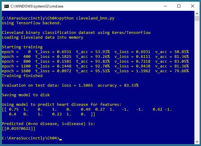
Figure 4-1: Binary Classification using Keras

The screenshot in Figure 4-1 shows a demonstration of binary classification. The demo program begins by loading 178 training data items, 59 validation data items, and 60 test data items into memory. Each item represents a patient who has heart disease (1) or not (0). There are 13 predictor variables in the raw data. After normalization and encoding, there are 18 input variables.

Behind the scenes, the demo program creates an 18-(10-10)-1 deep neural network, that is, one with 18 input values (one for each predictor value), two hidden layers both with 10 nodes, and a single output node. The demo program trains the neural network model using 2,000 epochs. During training, the loss and accuracy values for both the training data and the validation data are displayed.

After training completes, the trained model achieves a prediction accuracy of 83.33 percent on the test data (50 of 60 correct, 10 incorrect). The demo concludes by making a prediction for a new, hypothetical, previously unseen patient. The predicted probability is 0.0197, and because the value is less than 0.5, the output maps to 0, which in turn maps to a prediction of "no heart disease."

Understanding the data

The demo program uses the Cleveland Heart Disease dataset, a well-known classification benchmark dataset for statistics and machine learning. There are a total of 303 items. The raw data looks like this:

56.0,  1,  2,  120.0,  236.0,  0,  0,  178.0,  0,  0.8,  1,   3,   3,   0
62.0,  0,  4,  140.0,  268.0,  0,  2,  160.0,  0,  3.6,  3,   1,   6,   3
63.0,  1,  4,  130.0,  254.0,  0,  1,  147.0,  0,  1.4,  2,   2,   ?,   2
53.0,  1,  1,  140.0,  203.0,  1,  2,  155.0,  1,  3.1,  3,   0,   7,   1
[0]   [1] [2]  [3]     [4]    [5] [6]  [7]    [8]  [9]  [10] [11] [12] HD

The first 13 values on each line are the predictor values. The last value is 0 to 4, where 0 indicates no heart disease and 1 to 4 indicate heart disease of some kind. Predictor [0] is patient age. Predictor [1] is a Boolean sex (0 = female, 1 = male). Predictor [2] is categorical chest pain type encoded as 1 to 4.

Predictor [3] is blood pressure. Predictor [4] is cholesterol. Predictor [5] is a Boolean related to blood sugar (0 = low, 1 = high). Predictor [6] is categorical electrocardiographic result encoded as (0, 1, 2). Predictor [7] is maximum heart rate. Predictor [8] is a Boolean for angina (0 = no, 1 = yes). Predictor [9] is ST ("S-wave, T-wave") graph depression.

Predictor [10] is a categorical ST metric encoded as (1, 2, 3). Predictor [11] is a categorical count of colored fluoroscopy vessels encoded as (0, 1, 2, 3). Predictor [12] is a categorical value related to thalassemia encoded as (3, 6, 7).

The first step in data preparation is to deal with six data items that have one or more missing values. I took the simplest approach, which is to just delete any rows with missing data, leaving 297 data items. In my opinion, alternatives such as supplying an average column value, are usually not a good idea.

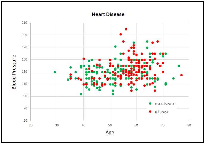
Figure 4-2: Partial Cleveland Heart Disease Data

The raw data was prepared by min-max normalizing the five numeric predictor variable values, by (-1, +1) encoding the three Boolean predictors, and by 1-of-(N-1) encoding the five categorical predictors. The class values-to-predict were encoded so that 0 means no indication of heart disease, and 1 means indication of some form of disease. I replaced the comma delimiters with tab characters.

After dealing with missing values, normalization, and encoding, the 297-item dataset was randomly split into three files: a 178-item (60 percent) set for training, and a 59-item (20 percent) set for validation, and a 60-item (20 percent) set for testing.

Because the Cleveland Heart Disease dataset has 13 dimensions, it's not possible to easily visualize it in a two-dimensional graph. But you can get a rough idea of the data from the partial graph in Figure 4-2. The graph shows only patient age and blood pressure for the first 160 items of the full dataset. As you can see, it's not possible to get a good prediction model using a simple linear technique like logistic regression or a base support vector machine linear model.

The Cleveland program

The complete program that generated the output shown in Figure 4-1 is shown in Code Listing 4-1. The program begins with comments the program file name (the _bnn is not a standard convention and just stands for binary neural network) and versions of Python, TensorFlow, and Keras used, and then imports the NumPy, Keras, TensorFlow, and OS packages:

# iris_dnn.py
# Python 3.5.2, TensorFlow 2.1.5, Keras 1.7.0
import numpy as np
import keras as K
import tensorflow as tf
import os
os.environ['TF_CPP_MIN_LOG_LEVEL']='2'

In a non-demo scenario, you'd want to include additional details in the comments. Because Keras and TensorFlow are under rapid development, it's a good idea to document which versions are being used. Version incompatibilities can be a significant problem when working with Keras and open-source software.

Code Listing 4-1: Cleveland Heart Disease Binary Classification Program

The program imports the entire Keras package and assigns an alias K. An alternative approach is to import only the modules you need, for example:

from keras.models import Sequential
from keras.layers import Dense, Activation

Even though Keras uses TensorFlow as its backend engine, you don't need to explicitly import TensorFlow, except in order to set its random seed. The OS package is imported only so that an annoying TensorFlow startup warning message will be suppressed.

The program structure consists of a single main function, with a program-defined helper class, MyLogger, for custom logging. The class definition is:

class MyLogger(K.callbacks.Callback):
  def __init__(self, n):
    self.n = n

  def on_epoch_end(self, epoch, logs={}):
    if epoch % self.n == 0:
      t_loss = logs.get('loss')
      t_accu = logs.get('acc')
      v_loss = logs.get('val_loss')
      v_accu = logs.get('val_acc')
      print("epoch = %4d  t_loss = %0.4f  t_acc = %0.2f%%  v_loss = %0.4f  \
v_acc = %0.2f%%" % (epoch, t_loss, t_accu*100, v_loss, v_accu*100))

The MyLogger class is used only to display loss and accuracy metrics that are computed automatically, so the class initializer doesn't need to accept references to the training data. Most program-defined callbacks would pass that information like this:

def __init__(self, n, data_x, data_y):
  self.n = n
  self.data_x = data_x
  self.data_y = data_y

The on_epoch_end() method pulls the current loss and accuracy metrics from the built-in logs dictionary and displays them. The demo program does this only so that the logging display messages can be reduced to once every 400 epochs instead of every epoch. Keras computes loss and accuracy for every training batch and averages the values over all batches at the end of each epoch. If you want more granular information, you can use the on_batch_end() method.

The main() function begins with:

def main():
  # 0. get started
  print("\nCleveland binary classification dataset using Keras/TensorFlow ")
  np.random.seed(1)
  tf.set_random_seed(2)

  # 1. load data
  print("Loading Cleveland data into memory \n")
  train_file = ".\\Data\\cleveland_train.txt"
  valid_file = ".\\Data\\cleveland_validate.txt"
  test_file = ".\\Data\\cleveland_test.txt"
. . .

In most situations you want your results to be reproducible. The Keras library uses the NumPy and TensorFlow global random-number generators, so it's good practice to set the seed values. The values used in the program, 1 and 2, are arbitrary. However, be aware that Keras program results typically aren't completely reproducible, due to order of numeric rounding of parallelized tasks.

The program assumes that the training, validation, and test data files are located in a subdirectory named Data. The purpose of the validation data is to monitor its loss and accuracy during training to prevent training the model too much, which could result in an overfitted model.

The basic idea is illustrated in the graph in Figure 4.3. The graph indicates that over time, loss/error on the training data will decline steadily. If you measure the loss/error on a hold-out set of validation data, you may be able to identify when model overfitting is starting to occur, and then you can stop training (known as "early stopping").

Although the train-validate-test idea is good in principle, in practice it usually doesn't work so well. The problem is that the loss/error values rarely drop in the nice, smooth way shown on the graph. Instead, the values tend to jump erratically, which makes identifying the start of model-overfitting very difficult.

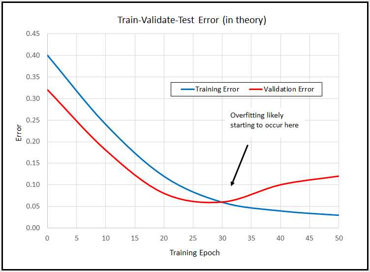
Figure 4-3: Train-Validate-Test in Theory

Additionally, holding out data for validation purposes reduces the amount of data you have for training. For these reasons, train-validate-test isn't very common. The demo program shows you how to use the technique because there are times when its useful, and so that you can understand it if you see it used.

The demo program doesn't have any information about the structure of the data files. I recommend that you include comments in your program that explain things such as how many predictor variables there are, types of encoding and normalization used, and so on. This kind of information is easy to remember when you’re writing your program, but difficult to remember a couple of weeks later.

The training, validation, and test data is read into memory with these statements:

  train_x = np.loadtxt(train_file, usecols=range(0,18),
   delimiter="\t",  skiprows=0, dtype=np.float32)
  train_y = np.loadtxt(train_file, usecols=[18],
    delimiter="\t", skiprows=0, dtype=np.float32)

  valid_x = np.loadtxt(valid_file, usecols=range(0,18),
   delimiter="\t",  skiprows=0, dtype=np.float32)
  valid_y = np.loadtxt(valid_file, usecols=[18],
    delimiter="\t", skiprows=0, dtype=np.float32)

  test_x = np.loadtxt(test_file, usecols=range(0,18),
   delimiter="\t",  skiprows=0, dtype=np.float32)
  test_y = np.loadtxt(test_file, usecols=[18],
    delimiter="\t", skiprows=0, dtype=np.float32)

In general, Keras needs feature data and label data stored in separate NumPy array-of-array style matrices. There are many ways to read data into memory, but the loadtxt() function is versatile enough to meet most problem scenarios. A common alternative approach is to use the read_csv() function from the Pandas ("Python Data Analysis Library") package. For example:

  import pandas as pd
  train_x = pd.read_csv(train_file, usecols=range(0,18),
    delimiter="\t", header=None, dtype=np.float32).values
  train_y = pd.read_csv(train_file, usecols=[18],
    delimiter="\t", header=None, dtype=np.float32).values

Notice that usecols can accept a list such as [0,1,2,3] or a Python range such as range(0,4). If you use the range() function, be careful to remember that the first parameter is inclusive, but the second parameter is exclusive.

In addition to the comma character, common values for the delimiter parameter are "\t" (tab) and " " (single space) The default parameter value is None which means any whitespace.

The default dtype parameter value is numpy.float, which is an alias for Python float, and is the exact same as numpy.float64. The default data type for almost all Keras functions is numpy.float32, so the program specifies this type. The idea is that for the majority of machine learning problems, the advantage in precision gained by using 64-bit values is not worth the memory and performance penalty.

Defining the neural network model

The demo program defines an 18-(10-10)-1 deep neural network using this code:

  # 2. define model
  init = K.initializers.RandomNormal(mean=0.0, stddev=0.01, seed=1)
  simple_adadelta = K.optimizers.Adadelta()
  X = K.layers.Input(shape=(18,))
  net = K.layers.Dense(units=10, kernel_initializer=init,
    activation='relu')(X)
  net = K.layers.Dropout(0.25)(net)  # dropout for layer above
  net = K.layers.Dense(units=10, kernel_initializer=init,
    activation='relu')(net)
  net = K.layers.Dropout(0.25)(net)  # dropout for layer above
  net = K.layers.Dense(units=1, kernel_initializer=init,
    activation='sigmoid')(net)

  model = K.models.Model(X, net)
  model.compile(loss='binary_crossentropy', optimizer=simple_adadelta,
    metrics=['acc'])

The demo sets up random Gaussian initial weights. Deep neural networks are often very sensitive to the initial values of the weights and biases, so Keras has several different initialization functions you can use.

The training optimizer object is Adadelta() ("adaptive delta"), one of many advanced variations of basic stochastic gradient descent. Selecting a Keras optimizer can be a bit intimidating. Table 4-1 lists five of the most commonly used optimizers.

Table 4-1: Five Common Keras Optimizers

One of the strengths of the Keras optimizers is that they all have sensible default parameter values, so you can try different optimizers very easily.

The demo program specifies each layer separately, and then combines them using the Model() method. An alternative approach is to use the Sequntial() method. The two approaches create the exact same neural network, but are quite a bit different in terms of syntax. The choice is one of personal preference.

The demo uses Dropout() layers. The purpose of Dropout is to reduce the likelihood of model overfitting. From a syntax point of view, you place a Dropout() layer immediately after the layer you wish to apply it to. The single parameter is the percentage of nodes in the affected layer to randomly drop on each training iteration. The advantage of using Dropout() is that it’s often effective in combating overfitting. The disadvantage is that you have to deal with additional hyperparameters to define where to apply dropout, and what dropout rate to use..

Note that it's possible to apply dropout to a neural network input layer; this is sometimes called jittering. However, using dropout on a neural network input layer is quite rare, and you should use it somewhat cautiously.

The demo program uses relu (rectified linear unit) activation for the hidden nodes. The relu activation function is often more resistant to the vanishing gradient problem, which causes training to stall out, than tanh or sigmoid activation.

The output layer, with its single node, uses sigmoid activation. This coerces the output node to a single value between 0.0 and 1.0, which can be interpreted as the probability that the target class is 1 (presence of heart disease in this problem). Put another way, if the output node value is less than 0.5, the prediction is class = 0 (no heart disease); otherwise, the prediction is class = 1 (heart disease).

The model is compiled with binary_crossentropy as the loss function. For multiclass classification, you can use categorical_crossentropy or mean_squared_error, but for binary classification problems, you can use binary_crossentropy or mean_squared_error.

The metrics parameter to compile() is optional. The demo program passes a Python list containing just 'acc' to indicate that classification accuracy (percentage correct predictions) should be computed for each batch during training.

Training and evaluating the model

After training data has been read into memory and the neural network has been created, the program trains the network using these statements:

  # 3. train model
  bat_size = 8
  max_epochs = 2000
  my_logger = MyLogger(int(max_epochs/5))
  print("Starting training ")
  h = model.fit(train_x, train_y, batch_size=bat_size, verbose=0,
    epochs=max_epochs, validation_data=(valid_x,valid_y),
    callbacks=[my_logger])
  print("Training finished \n")

The batch size is a hyperparameter, and a good value must be determined by trial and error. The max_epochs argument is also a hyperparameter. Larger values typically lead to lower loss and higher accuracy on the training data, at the risk of overfitting on the test data.

Training is configured to display loss and accuracy on the training data and the validation data every 2000 / 5 = 400 epochs. In a non-demo scenario, you'd want to see information displayed much more often.

The fit() function returns an object that holds complete logging information. This is sometimes useful for analysis of a model that refuses to train. The demo program does not use the h object, so it could have been omitted.

After training, the model is evaluated:

  # 4. evaluate model
  eval = model.evaluate(test_x, test_y, verbose=0)
  print("Evaluation on test data: loss = %0.4f  accuracy = %0.2f%% \n" \
    % (eval[0], eval[1]*100) )

The evaluate() function returns a Python list. The first value at index [0] is the always value of the required loss function specified in the compile() function, binary_crossentropy in this case. Other values in the list are any optional metrics from the compile() function. In this example, the shortcut string 'acc' was passed so the value at index [1] holds the classification accuracy. The program multiples by 100 to convert accuracy from a proportion (like 0.8234) to a percentage (like 82.34 percent).

Saving and using the model

In most situations you'll want to save a trained model, especially if the training took hours or even longer. The demo program saves the trained model like so:

  # 5. save model
  print("Saving model to disk \n")
  mp = ".\\Models\\cleveland_model.h5"
  model.save(mp)

Keras saves a trained model using the hierarchical data format (HDF) version 5. It's a binary format, so saved models can't be inspected with a text editor. In addition to saving an entire model, you can save just the model weights and biases, which is sometimes useful. You can also save the just model architecture without the weights.

A saved Keras model can be loaded from a different program like this:

print("Loading a saved model")
mp = ".\\Models\\cleveland_model.h5"
model = K.models.load_model(mp)

An alternative to saving the fully trained model is to save different versions of the model as they're trained. You could add the save code to the on_epoch_end() method of the program-defined MyLogger object, for example:

def on_epoch_end(self, epoch, logs={}):
  if epoch % self.n == 0:
    m_name = ".\\Models\\cleveland_" + str(epoch) + "_model.h5"
    self.model.save(m_name)

Keras also has a built-in ModelCheckpoint callback, which has parameters that allow you to do things such as saving only if a specified metric improves (lower loss, higher accuracy).

The demo program concludes by making a prediction:

  # 6. use model
  unknown = np.array([[0.75, 1, 0, 1, 0, 0.49, 0.27, 1, -1, -1, 0.62, -1, 0.40,
    0, 1, 0.23, 1, 0]], dtype=np.float32)
  predicted = model.predict(unknown)
  print("Using model to predict heart disease for features: ")
  print(unknown)
  print("\nPredicted (0=no disease, 1=disease) is: ")
  print(predicted)

Because the model was trained using normalized and encoded data, you must pass input values that have been normalized and encoded in the same way. Notice that the feature predictor values are passed as a NumPy array-of-arrays object.

The output prediction is raw in the sense that it's just a value between 0.0 and 1.0, and therefore, it's up to you to interpret the meaning. You can do so programmatically along the lines of:

labels = ["no indication of heart disease", "indication of heart disease"]
if predicted < 0.50:
  result = labels[0]
else:
  result = labels[1]
print(result)

Note that it is possible to perform binary classification by encoding the two classes-to-predict as (1, 0) and (0, 1), and then treating the problem as multiclass classification (softmax output layer activation and categorical cross entropy loss).

Summary and resources

To perform binary classification, you encode the target labels using 0-or-1 encoding. The number of nodes in the input layer is determined by the structure of your normalized and encoded data. The number of output nodes should be one, and the activation function on the output layer should be set to sigmoid so the node value is between 0.0 and 1.0, where a value less than 0.5 indicates a prediction of class = 0; otherwise, the prediction is class = 1.

The loss function should be set to binary_crossentropy, but you can use mean_squared_error if you wish. In general you should pass accuracy to the optional metrics list of the compile() function.

Free parameters for binary classification include the number of hidden layers and the number of nodes in each hidden layer, optimizer algorithm (Adagrad, Adadelta, and Adam are often good choices), batch size, and the maximum number of training epochs to use.

You can find the training, validation, and test data used by the demo program here.

The demo program uses a custom, program-defined callback class. See information about Keras built-in callbacks here.

This chapter described five of the most commonly used training optimizer algorithms. See information about all optimizers here.