Autoencoders

An autoencoder is a type of neural network that can perform dimensionality reduction for visualization. For example, suppose you have data that represents the age and height of men and women. If you want to graph your data, you can do so easily by plotting age on the x-axis and height on the y-axis, with blue dots for men and pink dots for women. But if your data has five dimensions, such as (age, height, weight, income, years-education), then there's no easy way to graph the data.

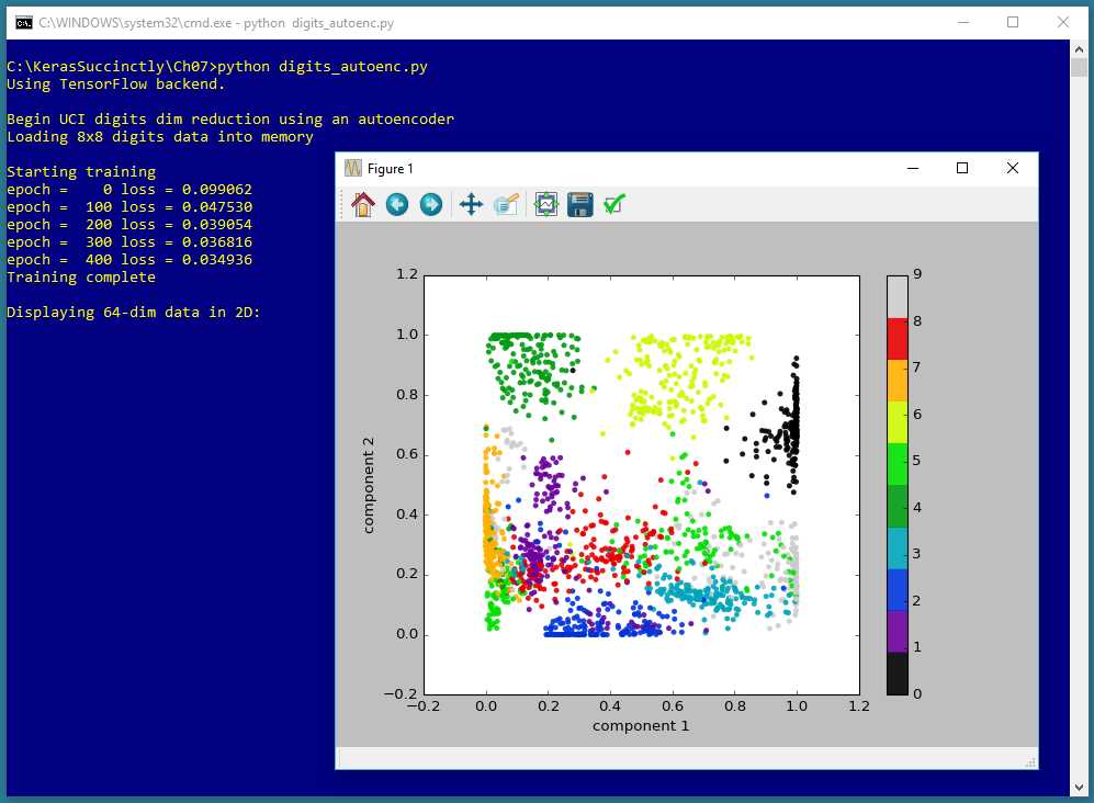
Figure 7-1: Autoencoder Dimensionality Reduction for Visualization using Keras

The screenshot in Figure 7-1 shows a demonstration of autoencoder dimensionality reduction for visualization. The demo program begins by loading 1,797 data items into memory. Each data item has 64 dimensions. The demo program creates an autoencoder that encodes/compresses each 64-dimensional data item down to two dimensions, and then graphs the result. Each of the data items belong to one of ten classes, and this information is used to color each point on the graph.

The 1,797 data items represent crude 8x8 bitmaps of handwritten digits from 0 to 9. In other words, the autoencoder visualization is applied to data that is itself a representation of a visualization. However, autoencoder dimensionality reduction for visualization can be applied to any type of data. For example, the Fisher's Iris dataset has four dimensions (sepal length, sepal width, petal length, and petal width), and the data could be reduced to two dimensions for visualization using an autoencoder.

Understanding the data

The demo data looks like this:

0,0,0,1,11,0,0,0,0,0,0,7,8, . . . 16,4,0,0,4
0,0,9,14,8,1,0,0,0,0,12,14, . . . 5,11,1,0,8
. . .

Each line of data represents a handwritten digit. The first 64 values on a line are grayscale pixel values between 0 and 16. The last value on a line is the digit value.

The screenshot in Figure 7-2 shows one of the data items. The data item is first displayed in the shell, using the raw pixel values expressed in hexadecimal. Then the item is displayed graphically.

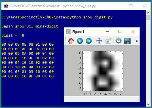
Figure 7-2: One of the UCI Digits

The goal of an autoencoder is to reduce the 64 dimensions of an item down to just two values so the item can be graphed as a point on an x-y graph.

The Autoencoder program

The complete program that generated the output shown in Figure 7-1 is shown in Code Listing 7-1. The program begins with comments for the program file name and versions of Python, TensorFlow, and Keras used, and then imports the NumPy, Keras, TensorFlow, PyPlot and OS packages:

# digits_autoenc.py
# Python 3.5.2, TensorFlow 2.1.5, Keras 1.7.0
import numpy as np
import keras as K

import tensorflow as tf
import matplotlib.pyplot as plt
import os
os.environ['TF_CPP_MIN_LOG_LEVEL']='2'

In a non-demo scenario, you'd want to include additional details in the comments. Because Keras and TensorFlow are under rapid development, you should always document which versions are being used. Version incompatibilities can be a significant problem when working with Keras and other open-source software.

Code Listing 7-1: Autoencoder Program

The program imports the entire Keras package and assigns an alias K. An alternative approach is to import only the modules you need, for example:

from keras.models import Sequential
from keras.layers import Dense, Activation

Even though Keras uses TensorFlow as its backend engine, you don't need to explicitly import TensorFlow, except in order to set its random seed. The OS package is imported only so that an annoying TensorFlow startup warning message will be suppressed.

The program structure consists of a single main function, plus a helper class for displaying messages during training. The helper class definition is:

class MyLogger(K.callbacks.Callback):
  def __init__(self, n):
    self.n = n   # print loss every n epochs

  def on_epoch_end(self, epoch, logs={}):
    if epoch % self.n == 0:
      curr_loss =logs.get('loss')
      print("epoch = %4d loss = %0.6f" % (epoch, curr_loss))

The MyLogger class is used to print the value of the built-in loss function every 100 epochs. The idea is that the fit() method can display progress messages every epoch, or not at all, but if you want messages every few epochs, you must define a custom callback class.

The main() code begins with:

def main():
  # 0. get started
  print("\nBegin UCI digits dim reduction using an autoencoder")
  np.random.seed(1)
  tf.set_random_seed(1)

  # 1. load data into memory
  print("Loading 8x8 digits data into memory \n")
  data_file = ".\\Data\\digits_uci_test_1797.txt"
  data_x = np.loadtxt(data_file, delimiter=",", usecols=range(0,64),
    dtype=np.float32)
  labels = np.loadtxt(data_file, delimiter=",", usecols=[64],
    dtype=np.float32)
  data_x = data_x / 16
. . .

In most situations, you want to make your results reproducible. The Keras library makes extensive use of the NumPy global random-number generator, so it's good practice to set the seed value. The seed value used in the program, 1, is arbitrary. Similarly, because Keras uses TensorFlow, you'll often want to set its seed, too. Unfortunately, program results typically aren't completely reproducible due to order of numeric rounding of parallelized tasks.

My preferred style is to indent with two spaces rather than the normal four spaces. All normal error-checking has been removed to keep the main ideas as clear as possible.

The program assumes that the training and test data files are located in a subdirectory named Data. The program itself doesn't have any information about the structure of the data files. I strongly recommend that you include in your program comments such as:

# data has 1797 items, is comma-delimited and looks like:
# 0,0,12,10, . . 13,11,5
# 0,0,0,2,8, . . 12,10,8
# first 64 values are grayscale pixel values between 0 and 16
# last value is the class label, '0' through '9'

This kind of information is easy to remember when you’re writing your program, but can be very difficult to remember a couple of weeks later.

The single data file is read into memory using the np.loadtxt() function. There are many ways to read data into memory, but the loadtxt() function is versatile enough to meet most problem scenarios. The NumPy genfromtxt() function is very similar but gives you a few additional options, such as dealing with missing data. The loadtxt() function has a large number of parameters, but in most cases, you only need usecols, delimiter, and dtype. 

Notice that usecols can accept a list such as [64] or a Python range such as range(0,64). If you use the range() function, be careful to remember that the first parameter is inclusive, but the second parameter is exclusive.

The default dtype parameter value is numpy.float, which is an alias for Python float, and is the exact same as numpy.float64. But the default data type for almost all Keras functions is numpy.float32, so the program specifies this type. The idea is that for the majority of machine learning problems, the advantage in precision gained by using 64-bit values is not worth the memory and performance penalty.

Instead of using a NumPy function such as loadtxt() to read data into memory, a different approach is to use the Pandas (originally "panel data," now "Python Data Analysis") library, which has many advanced data manipulation features. However, Pandas has a non-trivial learning curve and requires significant investment of your time.

After the digits pixel x-data has been loaded into memory, the data is normalized by dividing all values by 16. This makes all pixel values between 0.0 and 1.0, which makes the autoencoder a bit easier to train.

Defining the autoencoder model

The program defines a 64-32-2-32-64 autoencoder using this code:

  # 2. define autoencoder
  my_init = K.initializers.glorot_uniform(seed=1)
  X = K.layers.Input(shape=[64])
  layer1 = K.layers.Dense(units=32, activation='sigmoid',
    kernel_initializer=my_init)(X)
  layer2 = K.layers.Dense(units=2, activation='sigmoid',
    kernel_initializer=my_init)(layer1)
  layer3 = K.layers.Dense(units=32, activation='sigmoid',
    kernel_initializer=my_init)(layer2)
  layer4 = K.layers.Dense(units=64, activation='sigmoid',
    kernel_initializer=my_init)(layer3)

  enc_dec = K.models.Model(X, layer4)
  encoder = K.models.Model(X, layer2)

The architecture of an autoencoder for dimensionality reduction is best explained by a diagram—see Figure 7-3. The diagram shows a small 6-3-2-3-6 autoencoder rather than the large 64-32-2-32-64 architecture of the demo program.

There are two key ideas. First, an autoencoder's input and output are the same. Second, the inner-most layer has two nodes, which correspond to the x-axis and y-axis values for graphing.

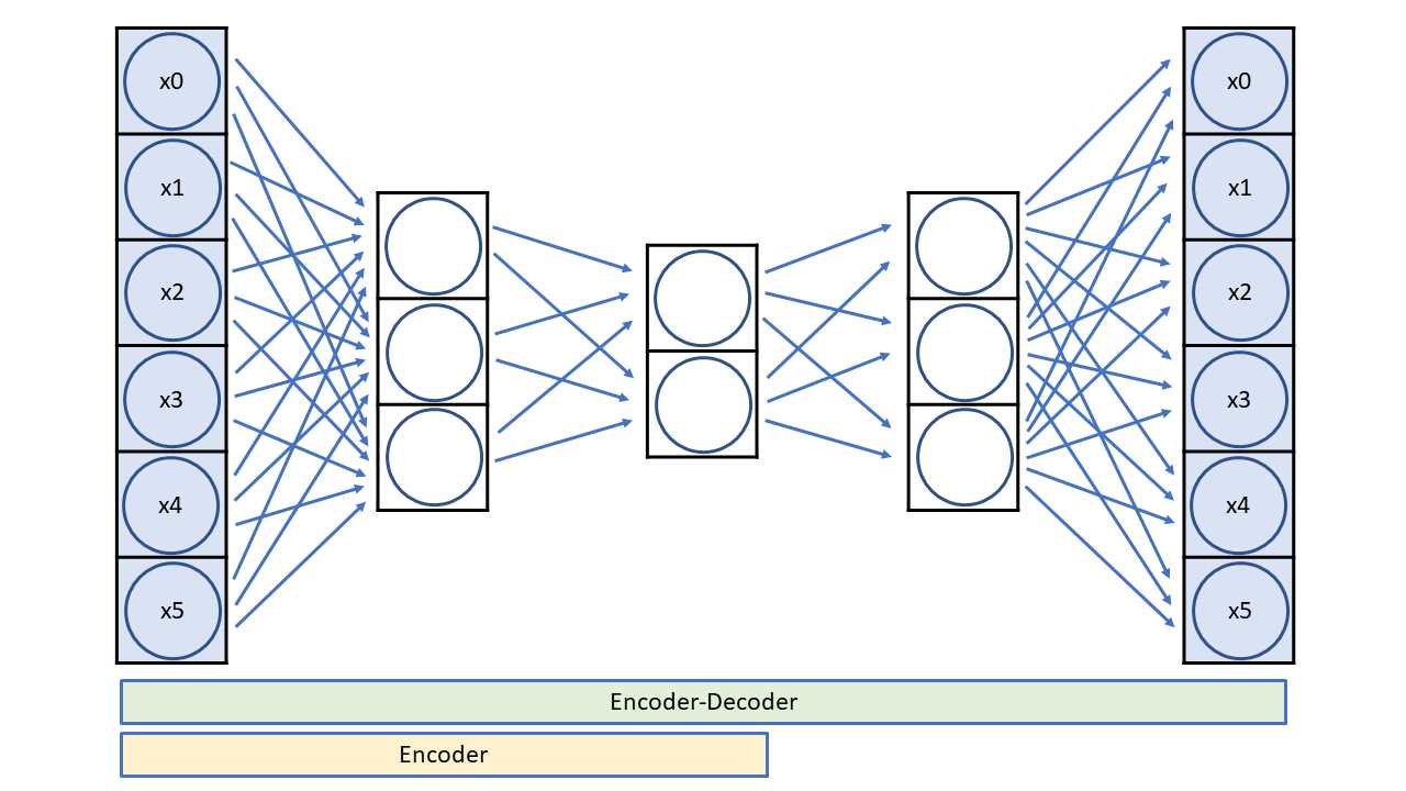
Figure 7-3: A 6-3-2-3-6 Autoencoder

An autoencoder is a special neural network that learns to predict its own input. After training, the inner-most two nodes are a reduced dimensionality representation of the input. An autoencoder is a specific type of neural network called an encoder-decoder. The encoder part of the network extracts the compressed representation of the network's input.

The number of autoencoder input nodes and output nodes is determined by the dimensionality of your data. The inner-most layer will usually have two or three nodes if the goal is dimensionality reduction for visualization. The number of other hidden layers and the number of nodes in each layer are free parameters.

Compiling and training the autoencoder

After training data has been read into memory and the autoencoder has been defined, the model is compiled and trained:

  # 3. compile model
  simple_adam = K.optimizers.Adam()
  enc_dec.compile(loss='mean_squared_error', optimizer=simple_adam)

  # 4. train model
  print("Starting training")
  max_epochs = 500
  my_logger = MyLogger(n=100)
  h = enc_dec.fit(x=data_x, y=data_x, batch_size=8, epochs=max_epochs,
    verbose=0, callbacks=[my_logger])
  print("Training complete \n")

The Adam (adaptive moment estimation) optimizer is a good general-purpose learner for deep neural networks, but Adagrad, Adadelta, and RMSprop are reasonable alternatives. Because the target values are type np.float32, the autoencoder is compiled using mean-squared error rather than cross-entropy error.

The number of training epochs and the batch size are free parameters. Notice that the fit() method is passed data_x for both the x and y parameters. The demo program captures the return object holding the training history from the fit() method, but doesn't make use of it. If you want to see the loss values, you can do so like this:

print(h.history['loss']) 

The verbose=0 parameter suppresses all built-in logging messages so that only the ones generated by the my_logger callback object are displayed.

Saving and using the autoencoder

In most situations, you'll want to save a trained model, especially if the training took hours or even longer. The demo program does not save the trained autoencoder, but you can do so like this:

  # save autoencoder model
  print("Saving model to disk \n")
  mp = ".\\Models\\autoenc_model.h5"
  encoder.save(mp)

Keras saves trained models using the hierarchical data format (HDF) version 5. It is a binary format, so saved models can't be inspected with a text editor. In addition to saving an entire model, you can save only the model weights and biases, which is sometimes useful. You can also save the model architecture without the weights.

A saved Keras autoencoder can be loaded from a different program like this:

print("Loading a saved model")
mp = ".\\Models\\autoenc_model.h5"
encoder = K.models.load_model(mp)

The demo program generates a two-dimensional visualization of the 1797 64-dimensional data items using these statements:

  # 5. generate (x,y) pairs for each digit
  reduced = encoder.predict(data_x)

  # 6. graph the digits in 2D
  print("Displaying 64-dim data in 2D: \n")
  plt.scatter(x=reduced[:, 0], y=reduced[:, 1],
    c=labels, edgecolors='none', alpha=0.9,
    cmap=plt.cm.get_cmap('nipy_spectral', 10), s=20)

  plt.xlabel('component 1')
  plt.ylabel('component 2')
  plt.colorbar()
  plt.show()

The call to the predict() method returns a NumPy array-of-arrays style matrix named reduced with 1797 rows and two columns, where column [0] is the x-axis value and column [1] is the y-axis value. The PyPlot scatter() function is used to generate a scatter plot.

The scatter() parameter names are a bit cryptic. Parameter c is a sequence of n numbers to be mapped to colors using the cmap parameter. Recall that array label holds the class labels 0 through 9 (as type np.float32) for each data item.

The cmap parameter ("colormap") has value 'nipy_spectral', which uses a continuous set of colors from dark purple, to green, to dark red. There are many other PyPlot colormaps, including 'rainbow', 'jet', 'Dark1', and 'cool'.

The s parameter controls the size (measured in points) of the marker dots on the scatter plot. The alpha parameter controls the transparency of the marker dots.

Summary and resources

An autoencoder is a special type of neural network that learns to predict its own input values. Because autoencoders don't use labeled data during training, autoencoders are an example of an unsupervised technique.

One common use of autoencoders is for dimensionality reduction, so that high-dimensionality data can be visualized on a two-dimensional or three-dimensional graph.

You can find the 1797-item data file used by the demo program here.

Other resources:

• Complete UCI digits dataset
• Reference for the PyPlot scatter function
• Colormap examples
• Reference for the Keras Model class API