Partitioning Data

Sharding data

Splitting a logical database object across multiple physical storage locations is the key to achieving high performance and scalability. The more storage locations, the more compute nodes can concurrently access the files. Intensive jobs can be run with a high degree of parallelism, which means they will run more efficiently and finish more quickly.

Some databases call this sharding, and the cost of the improved performance typically comes in the form of greater complexity in accessing the data. In some implementations you must specify which shard to insert or read from, and the administration—such as redistributing data if some shards become overloaded—is not trivial.

Hive supports two different types of sharding for storing internal tables—partitions and buckets. The sharding approach is specified when the table is created, and Hive uses column values to decide which rows go into which shard. This action abstracts some of the complexity from the user.

Sharding data is a key performance technique, and it is typically used in Hive for all but the smallest tables. We address it later in this book because we now have a good understanding of how Hive logically and physically stores and accesses data. Learning about sharding will be straightforward at this point.

Partitioned tables

Sharding a table into multiple partitions will physically split the storage into many folders in HDFS. If you create an internal Hive table without partitions, the data files will be stored (by default) in HDFS at /user/hive/warehouse/[table_name]. How you populate that table dictates how many files get created, but they will all be in the same folder.

Figure 6 shows how the syslogs table can be physically stored when it has been populated.

Figure 6: Folder Structure for an Unpartitioned Table

When we create a partitioned internal table, Hive creates subfolders for each branch of the partition, and the data files reside in the lowest-level subfolder. We specify how to partition the data, and the most efficient partition scheme will reflect the access patterns for the data.

If we typically load and query logs in batches for a particular date and server, we can partition the table by period and server name. As the table gets populated, Hive will create a nested folder structure using /user/hive/warehouse/[table_name] as the root and./[period]/[server] for the subfolders, as in Figure 7.

Figure 7: Folder Structure for a Partitioned Table

Creating partitioned tables

The create table statement supports a partitioned by clause in which you specify the columns used to partition the data files. You can specify multiple columns, and each will add another level of nesting to the folder structure.

For comparison, Code Listing 73 shows the structure of a table that is not partitioned, along with the structure of the folders in HDFS.

Code Listing 73: File Listing for an Unpartitioned Table

The two files in this listing contain different combinations of period and host, but because the table is not partitioned, the files are in the root folder for the table, and any file could contain rows with any period and host name.

Code Listing 74 shows how to create a partitioned version of the syslogs table.

Code Listing 74: Creating a Partitioned Table

Note: The columns you use to partition a table are not part of the column list, which means that when you define your table, you specify columns for all the data fields that are not part of the partitioning scheme, and you will specify partition columns separately.

As data gets inserted into the table, Hive will create the nested folder structure. Code Listing 75 shows how the folder looks after some inserts.

Code Listing 75: File Listing for a Partitioned Table

Here we have two folders under the root folder, with names specifying the partition column name and value (period=201601 and period=201602); beneath those folders we have another folder level that specifies the next partition column (host=sc-ub-xps and host=sc-win-xps).

In the partitioned table, the data files live under the period/host folder, and each file contains only rows for a specific combination of period and host.

Populating partitioned tables

Because rows in a partitioned table need to be located in a specific location, all the data population statements must tell Hive the destination target. This is done with the partition clause, which specifies the column name and value for all the rows being loaded.

The data being loaded cannot contain values for the partition columns, which means Hive treats them as a different type of column.

Code Listing 76 shows the description for the partitioned syslogs table in which the partition columns are shown as distinct from the data columns.

Code Listing 76: Describing a Partitioned Table

The data for the partition columns is still available to read in the normal way, but it must be written separately from other columns. Code Listing 77 shows how to insert a single row into the partitioned syslogs table.

Code Listing 77: Inserting into a Partitioned Table

The data to be inserted is split between clauses:

• PARTITION—contains the column names and values for the partition columns.
• VALUES—contains the values for data columns (names can be omitted, as in this example, which uses positional ordering).

If you try to populate a partitioned table without specifying the correct partition columns, Hive will raise an error.

Tip: This split between partition columns and data columns will add complexity to your data loading, but it ensures that every row goes into a file in the correct folder. If this seems odd at first, it's simply a case of remembering that columns in the partition clause of the create statement need to go in the partition clause for inserts, and they aren't included in the normal column list.

The partition syntax is the same for inserting multiple rows from query results, but here you need to ensure that you select only the appropriate rows for the target partition—you can't insert into many different partitions in a single load.

Code Listing 78 populates syslogs_partitioned by selecting from the syslogs table.

Code Listing 78: Selecting and Inserting into a Partitioned Table

Similarly, if the target table is partitioned, the load statement requires the partition clause. Apart from the partition columns, load works in the same way as we noted in Chapter 6  ETL with Hive—essentially it copies the source file to HDFS, using the partition specification to decide the target folder.

INSERT, UPDATE, DELETE

The key DML statements are only supported for ACID tables, but where they are supported the syntax remains the same as standard SQL. As of release 1.2.1, Hive supports some DML statements for tables that it does not recognize as ACID, as shown in Error! Reference source not found..

Table 3: DML Statement Support

Code Listing 79 creates a table that supports Hive transactions and specifies the ORC format, bucketed partitioning, and a custom table property in order to identify it as transactional.

Code Listing 79: Creating an ACID Table

In order to work with transactional tables, we need to set a range of configuration values. We can do this in hive-site.xml by making extensive use of transactional tables, or we can do this per session if we have only transactional tables.

The hive-succinctly Docker image is already configured in hive-site.xml in order to support the transaction manager, and it uses the following settings:

• "hive.support.concurrency" = "true".
• "hive.enforce.bucketing" = "true".
• "hive.exec.dynamic.partition.mode" = "nonstrict".
• "hive.txn.manager" = "org.apache.hadoop.hive.ql.lockmgr.DbTxnManager".
• "hive.compactor.initiator.on" = "true".
• "hive.compactor.worker.threads" = "1".

With the transaction settings configured, when we use DML statements with the ACID table, they will run under the transaction manager and we will be able to insert, update, and delete data. Code Listing 80: Inserting to an ACID TableCode Listing 80 shows the insertion of all the syslog data from the existing non-ACID table to the new ACID table.

Code Listing 80: Inserting to an ACID Table

If we want to modify that data, we can use update and delete on the table. As with SQL, Hive accepts a where clause in order to specify the data to act on. In Hive, the updates will be made in a map/reduce job, so that we can use complex queries and act on large result sets.

In Code Listing 81 we populate the hotspot column to identify processes that do a lot of logging, using a count query.

Code Listing 81: Updating an ACID Table

Now we can delete syslog entries for processes that are not hotspots, as in Code Listing 82.

Code Listing 82: Deleting from an ACID Table

This offers a straightforward way to identify that a minority of processes generates the majority of logs and leaves us with a table that contains the raw data for the main subset of processes.

Querying partitioned tables

Reading from partitioned tables is simpler than populating them because the partition columns are treated in the same way as data columns for reads, which means you can use the partition values in queries as well as the data values.

Code Listing 83 shows a basic select for all the columns in the syslogs_partitioned table, which will return all the partition columns and all the data columns without distinguishing between them.

Code Listing 83: Selecting from a Partitioned Table

You can also use a combination of partition and data columns in the selection criteria, as in Code Listing 84.

Code Listing 84: Filtering Based on Partition Columns

This query makes efficient use of the partitions in order to help distribute the workload. The where clause specifies a value for the period that will limit the source files to the folder period=201601 under the table root. There's a wildcard selection by host, so that all the files in all the host=sc-ub* folders will be included in the search.

Hive can split this job into multiple map steps, one for each file. Hadoop will run as many of those map steps in parallel as it can, given its cluster capacity. When the map steps are finished, one or more reducer steps collate the interim results, then the query completes.

Using partitioned tables correctly will give you a good performance boost whenever you read or write from the table, but you should think carefully about your partition scheme. If you use a large number of partition columns or partition columns with a wide spread of values, you might end up with a heavily nested folder structure that includes large numbers of small files.

It’s possible to reach a point at which having more files reduces performance because the extra overhead of running very large numbers of small map jobs outweighs the benefit of parallel processing. If you need to support multiple levels of sharding, you can use a combination of partitions and buckets.

Bucketed tables

Bucketing is an alternative data-sharding scheme provided by Hive. Tables can be partitioned or bucketed, or they can be partitioned and bucketed. This works differently from partitioning, and the storage structure is well suited to sampling data, which means you can work with small subsets of a large dataset.

With partitions, the partition columns define the folder scheme, and populating data in Hive will create new folders as required. With buckets, you specify a fixed number of buckets when you create the table, and, when you populate data, Hive will allocate it to one of the existing buckets.

Buckets shard data at the file level rather than the folder level, so that if you create a table syslogs_bucketed with five buckets, the folder structure will look like Figure 8.

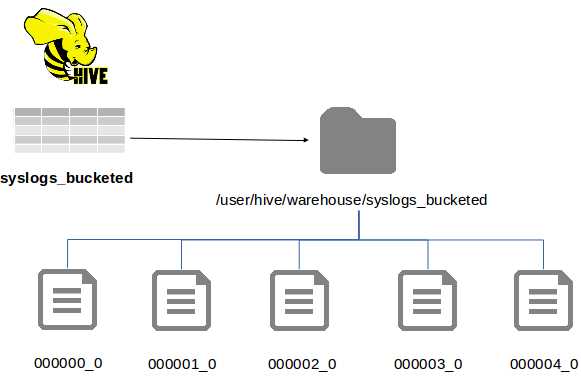
Figure 8: Folder Structure for a Bucketed Table

Here we still have the benefit of sharding data, but we don't have the issue of heavily nested folders, and we have better control over how many files the data is split across. Bucketed tables are also easier to work with because the bucket columns are normal data columns, which means we don't have to specify a partition when we load data.

Creating bucketed tables

The create table statement provides the clustered by … into buckets clause for sharding data into buckets. The columns used to identify the correct bucket are data columns in the table, which means they need to be specified in the usual way.

Code Listing 85 creates a bucketed version of the syslogs table using the period and host columns for the buckets. In this example the file is in ORC format, but that is not a requirement.

Code Listing 85: Creating a Bucketed Table

Note: The number of buckets is set to 12 here, which means Hive will allocate data between 12 storage locations. Rows with the same period and host will always be in the same location, but rows with different combinations of period and host can be in different buckets.

Hive doesn't create any folders or files until we start to populate the table, but after inserting a single row, the file structure for all the buckets will be created, as we see in Code Listing 86.

Code Listing 86: Folder Listing for a Bucketed Table

Tip: You can change the number of buckets for an existing table using the alter table statement with the clustered by clause, but Hive will not reorganize the data in the existing files to match the new bucket specification. If you want to modify the bucket count, it is preferable to create a new table and populate it from the existing one.

A subclause of clustered by directs Hive to create a sorted bucketed table. With sorted tables, the same physical bucket structure is used, but data within the files is sorted by a specified column value. In Code Listing 87 a variant of the syslogs table is created that is bucketed by period and host and is sorted by the process name.

Code Listing 87: Creating a Sorted Bucketed Table

Sorting the data in buckets gives a further optimization at read time. At write time, we can take advantage of Hive's enforced bucketing to ensure data enters the correct buckets.

Populating bucketed tables

When bucketed tables get populated, the storage structure is transparent, as far as the insert is concerned. Standard columns are used to determine the storage bucket, which means the standard insert statements work without any additional clauses.

The load statement cannot be used with bucketed tables because load simply copies from the source into HDFS without modifying the file contents. In order to support load for bucketed tables, Hive needs to read the source files and distribute the data into the correct buckets, which will lose the performance benefit of load in any case.

In order to populate bucketed tables, we need to use an insert. Code Listing 88 shows a simple insert into a bucketed table with specific values. Some key lines from Hive's output log are also shown.

Code Listing 88: Inserting into a Bucketed Table

The log entries from Beeline tell us that Hive used a single map task and 12 reduce tasks—one for each bucket in the table, which ensures data will end up in the right location. (Hive uses a hash of the bucketed column values to decide on the target bucket.) The table stats in the last line tell us there are 12 files but only one row in the table.

Data in a bucketed table can get out of sync, with rows in the wrong buckets, if the number of reducers for an insert job does not match the number of buckets. Hive will address that if the setting hive.enforce.bucketing is true in the Hive session (or in hive-site.xml, as is the case in the hive-succinctly Docker image).

With bucketing enforced by Hive, we don't have to specify which bucket to populate, and so we can insert data into multiple buckets from a single statement. In Code Listing 89 we take the formatted syslog rows from the previous ELT process in Chapter 6  ETL with Hive and insert them into the bucketed table.

Code Listing 89: ELT into a Bucketed Table

Querying bucketed tables

Bucketed tables are queried like any other tables, but query execution is optimized if the bucket columns are included in the where clause. In that case, Hive will limit the map input files to those it knows will contain the data, so that the initial search space is restricted.

There is no syntactical difference in queries over bucketed (or bucketed sorted) tables from tables which are not bucketed—Code Listing 90 shows a query using all the columns in the table.

Code Listing 90: Querying Bucketed Tables

Columns can be used in any part of the select statement irrespective of whether or not they are plain data columns or they form part of the bucketing (or sorting) specification.

Bucketed tables are particularly useful if you want to query a subset of the data. We've seen the limit clause in previous HiveQL queries, but that only constrains the amount of data that gets returned—typically the query will run over the entire table and return only a small portion.

With bucketed tables, we can specify a query over a sample of the data using the tablesample clause. Because Hive provides a variety of ways to sample the data, we can pick from one or more buckets or from a percentage of the data. In Code Listing 91 we fetch data from the fifth bucket in the bucketed syslogs table.

Code Listing 91: Sampling from Table Buckets

The entire table count returned 42 million rows in 21 seconds, yet a single bucket count took only three seconds to return 40,000 rows, which is significantly faster and tells me my data isn’t evenly split between buckets (if it was, I’d have about 3.5 million rows per bucket).

In order to sample a subset of data from multiple buckets, you can specify a percentage of the data size or a desired size for the sample. Hive reads from HDFS at the file block level, which means you might get a larger sample than you specified—if Hive fetches a block that takes it over the requested size, it will still use the entire block. Code Listing 92 fetches at least 3% of the data.

Code Listing 92: Sampling a Portion of Data

The efficient sampling returned with bucketed tables can be a huge timesaver when crafting a complex query. You can iterate over the query using a subset of data that will return quickly, and when you're happy with the query you can submit it to the cluster to run over the entire data set.

Summary

Sharding data is the key to high performance, and, because Hive is based on Hadoop, its core foundations support very high levels of parallelism. With the correct sharding strategy, you can maximize the use of your cluster—even if you have hundreds of nodes, they can all run parts of a query concurrently provided the data can be stripped to support that.

Hive provides two approaches to sharding that can be used independently or in combination. Which approach you choose depends on how your data is logically grouped and how you're likely to access it. Typically, the clauses you most frequently query over but which have a relatively small number of distinct values are good candidates for sharding—those might be time periods or the identifiers of source data or classifications for types of data.

Partitioned tables shard data physically by using a nested folder structure with one level of nesting for each partitioned column. The number of partitions is not fixed, and as you insert data into new partition column values, Hive will create partitions for you. Partition columns are a separate part of the normal table structure, which means your data loads are made more complex as they need to be partition aware.

The alternative to partitioned tables is bucketed tables that split data across many files rather than nested folders. The number of buckets is effectively fixed when the table is created, and standard data columns are used to decide the target bucket for new rows.

Bucketed tables are easier to work with because there is no distinction between the data columns and the bucket columns, and as Hive allocates data to buckets using a hash there will be an even spread with no hotspots if your column values are evenly spread. With bucketed columns you get the added bonus of efficient sampling in which Hive can pull a subset of data from one or more buckets.

Combining both approaches in a partitioned, bucketed table can provide the optimal solution, but you must select your sharding columns carefully.

In the final chapter, we'll look more closely at querying Hive and covering the higher value functionality HiveQL provides for Big Data analysis.