Programming Enterprise Hadoop in Windows

---

Hadoop performance and memory management within Windows Server

Consistency of Apache Hadoop builds across different Hadoop distributions is helpful, but doesn't mean that there'll be predictability of performance. In Windows, this can be both a blessing and a curse, but there are ways to ensure that it is a blessing.

Windows Server 2016 is a perfect partner for Hadoop from a technical perspective. It is capable of utilizing 256 processors, or 512 if Hyper-V is running. In addition, it can utilize 24 terabytes of RAM, or 12 on a virtual machine. In essence, it can handle any task that Hadoop may care to throw at it.

For this reason, I recommend that you use Windows Server for all the remaining exercises in this book. The only exception is if you use a local development cluster. In this case, you could use the latest version of Windows 10 Pro for Workstations, which can utilize four physical CPUs. Windows 10 Pro for Workstations and Windows 10 Enterprise could originally utilize only two physical CPUs. You would typically use the latest Windows 10 Pro for Workstations for local development, in conjunction with the multi-node cluster.

You'll need sufficient computing power to interrogate data after its ingestion into Hadoop. This doesn't just include dashboard creation tools, but also Relational Database Management Systems (RDBMS). All these tools must be running simultaneously, or you won't be able to connect to them live. This puts a load on both your network and the servers running within it. It's for these reasons that I detailed the hardware requirements earlier—Hadoop does not work in isolation in the real world.

In parts of the Hadoop ecosystem, like Hive, certain functions can be very resource intensive, such as creating joins between tables. Hive is not the only tool in which you can create joins but as it's a data warehouse I can' omit demonstrating it. Sadly Impala is not available within Windows and its near RDBMS query speed in Hadoop is has made it indispensable for many Linux users.

We'll be using IMDB (Internet Movie Database) data files for our exercises, and there are optional exercises for those happy to download 4GB of UK Land Registry data.

Let's examine how Hadoop in Windows will handle 4GB of data, and the kind of performance we could expect. We'll utilize part of what is known as “Amdahl’s law” to aid us in this.

Getting 4GB of data into Hadoop and processing it can be handled in a number of ways. It's partly dependent on the number of nodes you're using and the speed of your network. The aim is to process the data for use in dashboards or reports.

This can be expressed in the following ways:

• With four nodes, you could have four nodes processing 1 GB of data each.
• With eight nodes, you could have eight nodes processing 0.5 GB of data each.
• With 10 nodes, you could have 10 nodes processing 400 MB of data each.

Let's say the size of the data query results after processing is 4 MB. Let's look at what is going on behind the scenes to achieve that. It's those behind-the-scenes factors that will affect performance, even if your final data query results or output are small.

We know that networks don't quite reach their stated maximum speed, but let's assume you consistently reach 40 Mbps on a 1-Gbps network.

Table 8: Hadoop options for processing 4 GB of data

Table 8 shows that while your data can be processed faster, the time gains diminish the more nodes you add. The processing time drops from 25 seconds to 12.5 seconds when eight nodes are used instead of four. However, when 16 nodes are used instead of 12, data processing time only decreases by just over two seconds. Also, the data must be transported from more nodes to the node displaying the data, which adds to processing time. This leads to diminishing returns, to the point where adding more nodes becomes ineffective.

Another issue that’s just as important is how Hadoop stores data in a cluster—it stores them in blocks. Often the blocks are 128 MB or 64 MB, so a 4-GB file stored in 128-MB blocks is stored across 32 blocks. With each file in Hadoop being replicated three times, you then go from 32 to 96 blocks.

A further complication is that you can only store one file per block. Therefore, if your blocks are 64 or 128 MB, then files much smaller than those block sizes are highly inefficient. This is because a 1-MB file is stored in the same 128-MB block size as a 110-MB file. It also requires metadata about each block to be stored in the RAM. Luckily, you can alter block sizes for individual files to tackle this issue. There are also other file formats you can use, such as Avro and Parquet, that can greatly compress the size of your files for use in Hadoop. The benefits can be great, with query times well over ten or twenty times as fast as queries on the uncompressed file.

Once you get a feel for how Hadoop stores data, you can begin to estimate how much disk capacity and computing power your Hadoop project will require. While the metadata for each data block uses only a tiny amount of RAM, what happens to your RAM when you have hundreds, or even thousands, of files? The inevitable happens, and that small amount of memory is multiplied by thousands. Suddenly your RAM is compromised, and you feel the impact of file uploads on performance and memory management.

I would recommend actually carrying out calculations before considering the ingestion of large numbers of files. This enables a demarcation between system resources required for Windows servers in the cluster, and system resources they're losing to running Hadoop. In Windows, the monitoring of individual Windows servers can't be ignored. They are Windows servers in their own right, in addition to being part of a cluster. Where you have more demanding requirements, you can add more RAM to avoid encroaching the base RAM Windows Server needs. You may conclude that big data systems are in fact better at handling big data than small data, which should be no surprise. The problem is that by using compression too much, you can end up creating the very thing you don't want, which is too many small files.

While this isn't something that's done too often, I think it is important to isolate what is actually happening resource- and performance-wise when Hadoop is running in Windows. This informs answers to questions such as: Should Hadoop be the only application on each server? I take a particular interest in this, as Windows does not have the control groups (cgroups) feature that is available to Linux users. Cgroups can control and prioritize network, memory, CPU, and disk I/O usage. Cgroups also control which devices can be accessed and are in most major Linux distributions, including Ubuntu. Further features include limiting processes to individual CPU cores, setting memory limits, and blocking I/O resources. It is a feature that Windows Server does not have, and that Linux developers would notice. Without these features, we need to take care to monitor resource usage for Hadoop in Windows.

Let's start by looking at the resources used by the Big Data Platform within Windows Server. You could do this by setting up a virtual machine in Windows Server and allocating as little as 12 GB, though I'd feel safer at 16 GB, as a minimum. The reason for this is a simple one: it's the same reason that Linux and Microsoft list the minimum requirements for their operating systems as low as possible. If you list the minimum requirements as too high, you'll put off some customers and diminish the distribution or sale of your product. The trick is to be realistic and state recommended minimum requirements, as we'll do now. If you launch the Syncfusion Big Data Platform on a virtual or physical server with a realistic minimum of 16 GB of RAM, you will hopefully see the Resource Monitor in Figure 79. It shows Windows Server at only 22 percent CPU usage and 35 percent memory usage; this includes resources used running Windows Server.

Figure 79: Syncfusion Big Data distribution running in Windows Server 2016

Note that 22 percent of CPU usage is from processes, with 13 percent CPU usage from services, so there is low resource usage.

Figure 80: CPU processes and CPU services usage

At this point we have around 6 GB of memory in use by both Windows Server and the Big Data Platform, with approaching 3 GB on standby, and 7 GB free. Nearly 10 GB is available, which again, is stress-free computing. I am using i7 2.9 GHz CPUs, which are fast and robust processors.

Figure 81: Big data platform memory management on Windows Server

If we run the Cluster Manager as well as the Big Data product, and upload 1 GB of data files, the CPU usage goes up to as much as 37 percent, but the RAM behaves differently. Figure 82 shows that while memory usage is about the same 35-percent usage as before, the RAM use has gone down about 250 MB from the previous figure. More interestingly, the RAM on standby has increased to almost 5 GB, from under 3 GB. This decreases the amount of free RAM to under 5 GB. While 16 GB allows you to get up and running very comfortably, we know that for heavy lifting, we need 32 GB upwards. You have to act before—and not when—free memory runs out.

Figure 82: More RAM placed on standby leaving less free

I mentioned the IMDB data we'd be using to demonstrate data ingestion into the Syncfusion distribution of Hadoop. I am purposely using the .tsv file format for IMBD data and the .gz compressed file format.

The IMDB data is available from here.

Subsets of IMDB data are available for access to customers for personal and non-commercial use. You can hold local copies of this data, and it is subject to terms and conditions.

Download the zipped .gz files, then unzip the .tsv files using a tool like 7-Zip. The files include:

Title.basics.tsv.gz – contains the following information for film titles:

• tconst (string): Alphanumeric unique identifier of the title
• titleType (string):The type/format of the title (for example, movie, short, tvseries, tvepisode, video, etc.)
• primaryTitle (string): The more popular title, or the title used by the filmmakers on promotional materials at the point of release
• originalTitle (string): Original title, in the original language
• isAdult (boolean): 0 = non-adult title; 1 = adult title
• startYear (YYYY): Represents the release year of a title; in the case of a TV series, it is the series start year
• endYear (YYYY): TV series end year; \N for all other title types
• runtimeMinutes: Primary runtime of the title, in minutes
• genres (string array): Includes up to three genres associated with the title

Title.akas.tsv.gz – contains the localized film title:  

• titleId (string): A tconst, an alphanumeric unique identifier of the title
• ordering (integer): A number to uniquely identify rows for a given titleId
• title (string): The localized title
• region (string): The region for this version of the title
• language (string): The language of the title
• types (array): Enumerated set of attributes for this alternative title; can be one or more of the following: alternative, dvd, festival, tv, video, working, original, imdbDisplay. New values may be added in the future without warning.
• attributes (array): Additional terms to describe this alternative title, not enumerated

Title.episode.tsv.gz – contains the TV episode information:

• tconst (string): Alphanumeric identifier of episode
• parentTconst (string): Alphanumeric identifier of the parent TV series
• seasonNumber (integer): Season number the episode belongs to
• episodeNumber (integer): Episode number of the tconst in the TV series

Title.ratings.tsv.gz – contains the IMDB rating and votes information for titles:

• tconst (string): Alphanumeric unique identifier of the title
• averageRating (integer): Weighted average of all the individual user ratings
• numVotes (integer): Number of votes the title has received

We will also download UK Land Registry data, which is approaching 4 GB in file size. We require the 3.7-GB .csv file.

These include standard and additional-price-paid data transactions received at HM Land Registry from January 1, 1995 to the most current monthly data. The data is updated monthly, and the average size of this file is 3.7 GB, you can download the .csv file here. The data cannot be used for commercial purposes without the permission of HM Land Registry.

Hive data types and data manipulation language

One of the best sources of information on Hive data types and data manipulation language can be found here and here.

These two resources provide exhaustive information, whereas this section of the books lists essential information. Those of you who know SQL may find similarities between Hive data types and SQL data types; the same can be said for Hive Query Language and SQL.

Hive data types

Numeric types:

• TINYINT (1-byte signed integer, from -128 to 127)
• SMALLINT (2-byte signed integer, from -32,768 to 32,767)
• INT/INTEGER (4-byte signed integer, from -2,147,483,648 to 2,147,483,647)
• BIGINT (8-byte signed integer, from -9,223,372,036,854,775,808 to 9,223,372,036,854,775,807)
• FLOAT (4-byte single precision floating point number)
• DOUBLE (8-byte double precision floating point number)
• DOUBLE PRECISION (alias for DOUBLE, only available starting with Hive 2.2.0
• DECIMAL: Introduced in Hive 0.11.0 with a precision of 38 digits Hive 0.13.0 introduced user-definable precision and scale
• NUMERIC (same as DECIMAL, starting with Hive 3.0.0)

Date/time types:

• TIMESTAMP (Only available starting with Hive 0.8.0)
• DATE (Only available starting with Hive 0.12.0)
• INTERVAL (Only available starting with Hive 1.2.0)

 String types:

• STRING
• VARCHAR (Only available starting with Hive 0.12.0)
• CHAR (Only available starting with Hive 0.13.0)

Misc types:

• BOOLEAN
• BINARY (Only available starting with Hive 0.8.0)

 Complex types:

• arrays: ARRAY<data_type>
• maps: MAP<primitive_type, data_type>
• structs: STRUCT<col_name : data_type [COMMENT col_comment], ...>
• union: UNIONTYPE<data_type, data_type, ...>

Hive DML (Data Manipulation Language) provides support for:

                                   

• Loading files into tables
• Inserting data into Hive tables from queries or sub-queries
• Dynamic Partition Inserts
• Writing data into the filesystem from queries
• Inserting values into tables from SQL
• Updates
• Deletes
• Merges
• Joining of tables
• Grouping or aggregating the values of columns

Hive DDL (Data Definition Language) provides support for the following:

• Create database
• Describe database
• Alter database
• Drop database
• Create table
• Truncate table
• Repair table

                  

DDL functions also apply to the components of databases such as views, indexes, schemas, and functions. The best way of detailing or describing the terms and functions shown previously is to actually use them. To achieve this in Hadoop for Windows, we need to prepare our environment for data ingestion.

Enterprise data ingestion and data storage

To prepare our Hadoop environment for data ingestion and storage, launch the Syncfusion Big Data Studio and select the HDFS menu item. You'll notice in Figure 83 that there are some directories within Big Data Studio that are automatically loaded upon installation. There is also an Add Cluster button underneath the Clusters section. Underneath this button is the text localhost, which is the local development cluster installed automatically when you installed Big Data Studio. As we wish to connect to our multi-node cluster, let’s click the Add Cluster button.

Figure 83: Add Cluster to Syncfusion Big Data Studio

We need to enter the IP address of the host name of the active name node of our cluster. Enter the host server name or IP address as requested. In Figure 83, the full computer name (including domain element) is given, and it connects to the cluster, as seen in Figure 84.

Figure 84: Connecting to Hadoop cluster

The cluster is shown underneath the localhost cluster. To start receiving data, click New to add a new folder, enter a name for the folder, and click Create.

Figure 85: Creating a new folder on a cluster

You can also switch to your local cluster and create a folder there, by selecting the localhost cluster and clicking Start Services.

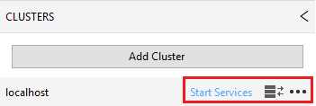
Figure 86: Starting services on the local cluster

This means you can switch between clusters by simply connecting or disconnecting.

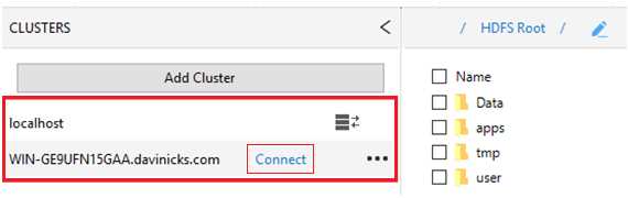
Figure 87: Option to switch between clusters

We are now going to do our first data upload to Hadoop. We are going to upload the 3.7-GB .csv file of house prices paid transactions mentioned earlier in the chapter. If you can't get ahold of the file, just follow along, as we'll be using files of a much smaller size in the next section. In Big Data Studio, choose the HDFS menu item. Click New to create a new folder, and call it ukproperty. It will appear to the right of the text HDFS Root, which is shown in Figure 88.

If you click ukproperty, you will access the folder. Once there, you can create another folder called 2018Update. You will now notice that the 2018Update folder has been added to the right of ukproperty, and if you click 2018Update, you will access that folder.

Next to the New folder button on the menu, click Upload and choose the radio button to select File. Use the button highlighted in the red rectangle in Figure 88 to select the property transactions file we are going to upload, called pp-complete.csv. Once you find and select the file, click OK, and you will see the following screen again. Now, click Upload.

Figure 88: Selecting file for HDFS upload

On the bottom, right-hand corner of the screen, you will see a box that shows a progress bar of the file uploading. When the file has been uploaded, it shows Completed.

Figure 89: File upload complete

The file should not take long to upload on a fast system, but you could be waiting a few minutes on a slower one. Hadoop for Windows benefits from fast, interactive facilities that are unavailable in many Windows applications. For example, I could not even begin to load a file this size into Excel. In QlikView, you'd be using all sorts of built-in compression (QVDs) to load the file, and your system would certainly feel it. In databases, you'd be taking a while to upload it, and then have to wait for running queries to view outputs from it. In Hadoop for Windows, this file is trivial on a powerful system. Simply double-click the uploaded file pp-complete1.csv, or right-click it and click View. The 4-GB file instantly opens in the HDFS File Viewer, which allows you to instantly go to any one of the 31,573 pages that make up the data file.

Figure 90: Instant viewing of 4-GB data fie in HDFS File Viewer

For these reasons, Hadoop for Windows is very useful for storing large files—you don't have to wait even a second to see what is contained in the large file you're viewing. Imagine quickly double-clicking on a 4-GB CSV file in Windows, and locking up your machine and whatever application tried to open it. In Hadoop for Windows you can have all your files, folders, and directories neatly ordered and instantly available to view. We will be using this 4-GB file a bit later in the book when we undertake some tasks of greater complexity.

We have ingested the data in HDFS, and we can store it and view it instantly in Windows. This is fine, but there is also a need to manipulate data once it's in HDFS. This is where the Hive data warehouse is used, along with other tools in the Hadoop ecosystem. We have to be able to use Hive in Windows to the same standard that Linux users use Hive in Linux.

Executing data-warehousing tasks using Hive Query Language over MapReduce

We're going to start by using lateral thinking, and show you something that appears to work, but doesn't really. It shows that the greatest strength of Hadoop can also be its greatest weakness, and how to avoid such pitfalls.

Create a new folder called Hadoop4win in the HDFS root folder, then upload the unzipped title.akas.tsv.gz IMDB file and name it titleaka.tsv in HDFS. Now, access the Hive data warehouse by selecting Hive from the menu in Big Data Studio.

Code Listing 15

Enter the code from Code Listing 15 in the Hive editor window, and then click Execute. The Hive editor window and console window are shown in Figure 91.

Figure 91: Hive Editor and Hive Console windows

The results are shown in the following figure.

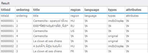
Figure 92: First results returned in Hive

We can remove the first row of data by using the code in Code Listing 16, and then clicking Execute.

Code Listing 16: Removing first row of data from table

The next figure shows the first row of data removed.

Figure 93: First line of duplicated header text removed in Hive

While these results may look okay, try clicking on the menu item Spark SQL. You'll now be asked to start the Spark thrift server; click the button presented to start it. After it starts, you'll see a panel on the right-hand side of the screen; click Databases at the bottom of the panel, and you'll see a section at the top of the panel called DataBase. This is shown in Figure 93.

Figure 94: Spark SQL environment

You then see a database called default and a database table called titleaka, as seen in Figure 94. It's the table we created in Hive that's now visible in Spark SQL. Right-click the titleaka table and click the option to Select Top 500 Rows. In the Spark SQL window, we can clearly see all the data was wrongly ingested into the titleId field; this is shown in Figure 95. The data looked correct in Hive, but it clearly isn't—imagine trying to use the table in a join with another table. As Hadoop can ingest so many different formats of data, there's a potential for errors in processing such a range of file formats.

Figure 95: Data fault clearly highlighted in Spark

Hadoop in Windows includes the ability to ingest data in compressed format, as you can with Hadoop in Linux. We are going to upload the IMDB data files title.episode.tsv.gz and title.ratings.tsv.gz to HDFS in compressed form. After we upload the files to the Hadoop4win folder, rename the title.ratings.tsv.gz file to title.rating.tsv.gz by right-clicking it and choosing Rename. The files as seen in HDFS (Figure 96) are smaller, as they are compressed. It's good for storage, since we don't have to decompress the files and use more space. Even better, we can work off those compressed files as if they were in an uncompressed state.

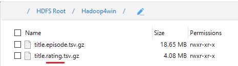
Figure 96: Uploaded compressed files in HDFS with title.ratings changed to title.rating

Enter the following code in the Hive editor window to create a table called titleepisode from the compressed title.episode.tsv.gz file.

Code Listing 17: Creating table in Hive from compressed file

Now, do the same to create a table called titlerating with the following code.

Code Listing 18: Code for creating second table from compressed file in Hive

The output in the next figure shows the output from the table created in the preceding code, namely select * from titlerating LIMIT 25. This selects the first 25 rows from the titlerating table we just created from the compressed file. This line is a good starting point for explaining the concept of MapReduce.

Figure 97: Rows returned from the select query

The query select * from titlerating LIMIT 25 does not make use of either map or reduce. This is because the select *, which means select all, runs through and returns values from all the columns. There is no filtering in use, which is basically what the map element of MapReduce is. In addition, there's no grouping of text or value data, so there's no aggregation or summing of values. This means there is no reduction, either.

Let’s put the two tables together in a join. Joins require tables to have individual columns filtered as columns to join tables on, so mapping is often a necessity. Resulting data from queries involving joins often have grouped elements, or indeed group aggregation, so reduction is also present in the query. This means that when using the Hive query language, certain queries will not quickly return your data set. Instead, you will see map and reduce actions running before your data set is returned.  Hive is often criticized for slow-running queries involving joins, and this is not without merit. It's also why Impala has become so popular; we will look at Impala a bit later. That said, a data warehouse not capable of executing joins is no data warehouse at all.

Let's join the tables after switching to Tez mode in Hive, which helps to speed up queries. Tez is not as fast as Impala by any means, but can make the difference between a query executing and a query failing.

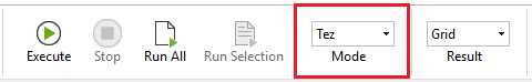
Figure 98: Switching to TEZ mode in Hive

This is achieved by clicking the Mode drop-down menu, as highlighted in Figure 98, and clicking TEZ instead of MR (MapReduce). Now, run the following code to join the two tables.

Code Listing 19: Code to join titlerating and titleepisode tables in Hive

After running this code, you'll notice a long delay before your results are returned, as the map and reduce actions are carried out, as shown next.

Figure 99: Map and Reduce actions in TEZ mode

Once the map and reduce actions are complete, the results of the joined tables are displayed.

Figure 100: Query results from joining titlerating and titleepisode tables using TEZ and MapReduce

Utilizing Apache Pig and using Sqoop with external data sources

Compared to the complexities of MapReduce, Pig is seen as more straightforward and economical to use in terms of lines of code required to achieve a task. It follows that the less code there is, the easier it is to maintain. It's important to note that MapReduce is still utilized within Pig, but the more literal way of expressing code in Pig is favored by many. If there was a negative, it would be that while the Hive query language and SQL have clear similarities, Pig really is a language of its own. You may not have used a language that looks or works anything like it. The differences with Pig are not just in its form, but in its execution, as it doesn’t need to be compiled.

To access Pig, simply click the Pig item from the menu in Big Data Studio. Create a folder within the Hadoop4win folder called titles, and unzip and upload the title.basics.tsv.gz file, and call it titlebasic.tsv. Now, enter the code from Code Listing 20 in the Pig editor window.

Code Listing 20: Code for grouping data in Pig

After you enter the code in the editor, you will notice the code created in the console. An important line in that code is the URL to track the job, as highlighted next.

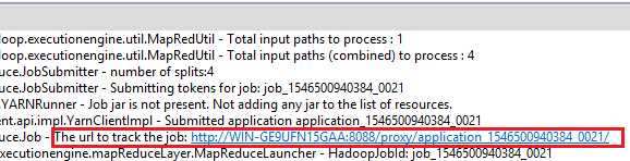
Figure 101: URL to track job in Pig

You simply click on the link shown, and you'll see an image similar to the one in Figure 102. The figure shows the same job as in the URL, which is 1546500940384_0021. It shows that the job succeeded and the time, date, and elapsed time. It also shows the map, shuffle, merge, and reduce time.

Figure 102: Tracking Pig MapReduce job

The requested result is also shown in the results window, which groups the individual start years of the films in the database.

Figure 103: Returned results of Pig query showing the start years of films in the IMDB.

Some people have preferences for Hive, and others for Pig; it can depend on what exactly you’re doing. Other people prefer to export their data out of Hadoop to work with relational database systems. This can be because they're much faster when working with joins between tables than Hadoop, for example. There’s no real difference when using Pig in Windows to using Pig with Hadoop in Linux. It’s therefore a good time to move onto Sqoop, which can import and export data to and from Hadoop. This is a key feature of Hadoop, and is available in Hadoop for Windows.

Sqoop

Because of current advances in integrating Hadoop in Windows, this section nearly failed to make the book. It would though be wrong to exclude it though, since it is used by so many people in Hadoop to import and export data. To access Sqoop, simply click Sqoop on the Big Data Studio menu. You'll notice in the following figure that the JDBC connectors are not installed. If you are able to go online, click the checkbox to select the Microsoft SQL Server JDBC Connector, and the highlighted Install button will become enabled. Click Install if you choose to install the driver in this fashion, or click the link highlighted in Figure 104 to get the instructions to install the connector jars manually.

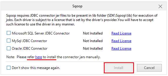
Figure 104: JDBC connector is not installed

As I am working with SQL Server v-next CTP 2.0 2019 Technology preview, I needed to download a connector that would work with it. So if you download sqljdbc_6.0.8112.200_enu, sqljdbc_7.0.0.0_enu or any other version it depends on the version of SQL Server you are using. You need to visit the Microsoft.com website to accurately determine this. One you extract the files you take the jar file which in my case is sqljdbc42 and place it in the Sqoop\lib folder. So in a multi-node cluster environment you place that file on each node where Sqoop is installed. The directory you place it in should be:

<InstalledDirectory>\Syncfusion\HadoopNode\<Version>\BigDataSDK\SDK\Sqoop\lib

If you are working on a local development cluster, the directory you should place it in is:

<InstalledDirectory>\Syncfusion\BigData\<Version>\BigDataSDK\SDK\Sqoop\lib

Figure 105: Connector Jar in the Sqoop\lib folder.

After you put the file in the relevant folder, close the Big Data Studio, and then open it again. The JDBC connector for SQL Server is now installed, as shown in Figure 106.

Figure 106: SQL Server JDBC Connector is now installed.

Click Add Connection, as shown in Figure 107, and insert the details for your own SQL Server system. Choose the title of the connector, the connector for SQL Server, and the connection string for your server. I named the title for my connector SqoopMov02 . Then put in the username and password for your SQL Server account; I'm using the SQL Server systems administrator account I set up in SQL Server. Next, click Save.

Figure 107: Creating a connection to SQL Server in Sqoop.

After saving the connection click Add Job and name the job CurrencyImport. Choose the connection SqoopMov02 from the drop-down box, as shown in Figure 108.

Figure 108: Adding new job in Sqoop

Since we're doing an import, click the Import radio button, then click Next. Now we will enter the details of the database and the table in SQL Server that we wish to import data from, as shown next. The database in SQL Server is called INTERN28, and the table is called Currencies. Click Next to continue.

Figure 109: Identifying database and table for data import

We now need enter the HDFS directory that we want the data imported into; in my case it's /Hadoop4win/data. Now, click the Save & Run button.

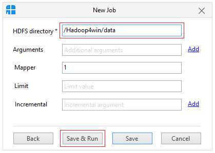
Figure 110: Save and run import job in Sqoop

You now see that the job is accepted, as reflected in the following figure.

Figure 111: Accepted Sqoop job

The status of the job then changes from Accepted to Succeeded.

Figure 112: Successfully completed Sqoop job

We now need to go the directory where we wanted the data imported to called /Hadoop4win/data. There you see the _Success notification, and underneath that, you see the table that has been imported, referenced part-m-00000. Double-click on it, and you see data we imported via the HDFS File Viewer. Notice that the file arrived first at 22:56:49, and then the success notification arrived a second later, at 22:56:50.

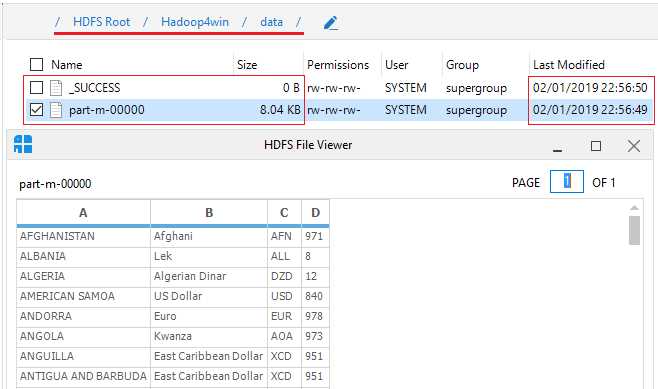
Figure 113: Sqoop data arrived successfully

Now let's do a Sqoop export; we'll use a file that's installed when you install the Syncfusion Big Data Studio. It's the Customers.csv file in the Customers folder, as shown in Figure 114.

Figure 114: Customers csv file that is installed with the software

We'll add a job as we did with the data import, but this time we choose the Export option. We'll use the same SqoopMov02 connection as we used for the import, as shown in the following figure. Now, click Next.

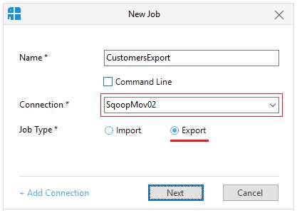
Figure 115: Starting an export job in Sqoop

We’ll use the button highlighted in Figure 116 to choose the folder we wish to export data from; here, it's Data/Customers/. Click Next.

Figure 116: Specifying folder to export data from

We now enter the name of the database we want to export the data to, and the name of the table we want to export the data to, and click Save & Run.

Figure 117: Save and run an export job in Sqoop

We now see the Succeeded status of the CustomerExport job shown under the previous successful CurrencyImport job. It shows that both jobs used the same Connection, as seen in Figure 118.

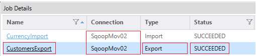
Figure 118: Sqoop export job succeeded

You should now also see the data exported from Sqoop in SQL Server, as displayed in the following figure. The customers.csv file data has arrived in the INTERN28 database table called Table_1.

Figure 119: Exported table from Syncfusion Hadoop distribution arrived in SQL Server

While Sqoop can import and export data, I can't say it's the smoothest or most efficient tool I've ever seen. This is nothing to do with Windows or Linux; I've just never felt it's an impressive tool. Fortunately, Microsoft is making real progress at integrating Hadoop with Windows, and this is providing alternatives. We will look at this in more depth in Chapter 4.                                                                                                                                                                                    

Summary

We started by presenting the capabilities of Windows Server as a perfect partner for Hadoop. Its ability to utilize 24 terabytes of RAM and 256 processors allow it to scale to any task that Hadoop can throw at it. We then used Amdhal’s Law to examine how Hadoop transports data across a network, and the mechanisms Hadoop uses to store and access data on disk.

We examined the system resources required by Hadoop in Windows Server, before looking at Hive data types and the Hive data manipulation language. We prepared Hadoop to ingest data as we began to upload files, create tables, and manipulate data in the Hadoop ecosystem. We manipulated compressed data files and executed table joins in Hive before carrying out jobs in Pig and setting up connections in Sqoop. This included loading external SQL Server drivers and focusing on the role of MapReduce in querying data in Hive and Pig.

We concluded by creating both import and export jobs between SQL Server and Sqoop after setting up Sqoop connections for data transfer. I think we can safely say that Hadoop and its ecosystem run perfectly on Windows Server—we are not missing out on anything in Windows that is available in Linux.

When we go one step further—to connect to and report from Hadoop—we see the advantages of the Windows environment over Linux. If you had asked me about this even a short while ago, I would not have agreed. Luckily, the release of the SQL Server v-next CTP 2.0 Technology Preview has changed all that.