Spatial SQL

---

I've mentioned this breed of SQL many times in this book, and to some extent I've also described it in a brief fashion.

Spatial SQL is not anything special; if you take "Spatial" out of the name, it's just regular SQL. Either way you're dealing with binary large objects, or blobs.

Just like working with images embedded in the database, these blobs have a special meaning when processed by code that understands what they contain. It's the addition of this code along with the extra SQL functions needed to use it that makes a spatially enabled database.

In the following section, I'm not going to cover every possible permutation and function call. At last count there are more than 300 independent functions in the OGC specification, covering just about every possible scenario from spatial distance relationships, to constructions of complex geometries, to clipping rasters for predefined vector paths.

Instead, using the data we've placed in our database, I'll guide you through some simple but common operations—the type that anyone writing a GIS-enabled application is likely to use.

Before we discuss these operations, let's take a quick look at the input and output stages described in the first chapter.

Creating and Retrieving Geometry

Even though we've already imported some data into our database, anyone writing a GIS app also needs to be able to create geometry in the database, especially if the application is going to allow editing.

Most geometry creation is performed in one of three formats:

• Well-known text (WKT)
• Extended well-known text (EWKT)
• Well-known binary (WKB)

We'll be using WKT in the examples that follow, and we'll only be performing the operations in SQL without inserting any data into our database. EWKT is slightly different, mostly due to the fact that in the textual representation of the geometry, the SRID is separated from the rest of the data by a semicolon.

I prefer to use the WKT standard and the spatial function ST_SetSrid to set the SRID for my geometries.

If you are using MS SQL, you may have to use EWKT since it doesn't have a ST_SetSrid function. There is, however, a writable SRID property on the Geometry SQL type.

So how do we create a geometry using WKT? Try the following SQL:

This creates a four-segment linestring that starts at 1,1, ends at 4,4, and passes through 2,2 and 3,3. The following is another example of creating geometry with SQL:

This creates a point at 5, 6 in the current coordinate system.

You can include an optional second parameter that specifies the SRID of the geometry. So if we wanted to create our point in OSGB36 (SRID 27700) coordinates, we'd use the following:

If you try this using the SQL editor in pgAdmin, you'll find that the database doesn't complain about the coordinates not being valid for the coordinate system being used. That's because the second parameter only sets the field in the geometry blob to say what the geometry's coordinate system is; it does not set anything in the metadata tables or anywhere else in the system to mark that SRID.

Please also note that if you are trying to insert these geometries into a table you have created, the triggers and constraints on those tables will have been set by the table creation functions to allow only certain geometry types and SRIDs to be inserted. This can disrupt many new GIS developers. If the second parameter is not specified, the database will set it to the table default. It's all too easy to insert an invalid coordinate if you don't specify the SRID.

If you do specify the SRID, but it doesn't match the SRID of the table you are inserting the geometry into, then the insert will be rejected and not committed to the table. It is very important to be sure when creating new geometries by hand that you have the correct SRID for your data, and that it matches the constraints of any tables you may have created.

Any of the geometry types we discussed in Chapter 1 can be used in the GeomFromText function, but beware as sometimes things are not quite as simple as you may expect, especially when it comes to MULT geometries.

The following is a simple point type.

Multipoints, on the other hand, look like this:

As you can see, simple parenthesis nesting can quickly become a nightmare. Some of the most bizarre bugs I've had to track down in GIS were a direct result of a missing parenthesis.

The same format is used for all other geometry types too.

The exception to the rule is polygons. Because polygons can include inner rings, a standard polygon actually looks like a single multipolygon from the start. This means that multipolygons have three sets of parentheses surrounding them.

This is not very nice to debug. Using a library like DotSpatial or SharpMap helps tremendously because it has functionality built in that allows you to use a familiar C# or VB object and have this text, or even a direct WKB representation, generated on the fly for you so you won't have to construct these geometries by hand.

There are other input functions besides GeomFromText. Most of them mirror the equivalent output functions listed in the next section. For your reference, I've listed some of the input functions available in the latest version of Postgres:

Other geometry functions available in the latest version of Postgres include:

All of which are detailed in the Geometry Constructors section of the online PostGIS manual at http://postgis.refractions.net/docs/reference.html#Geometry_Constructors. Most of the geometry constructors are also defined in the OGC specifications.

Output Functions

Now that we've seen how to generate geometry objects, it would be great to be able to get our data back out of the database.

If you want just the binary blob representation, a simple Select will do the job. In the creation samples in the previous section, because we weren't inserting the data, the output was the actual binary blob that represented the geometry.

One thing you must be cautious of: when dumping the blob directly, it might not be a WKB formatted object. Some database services store the data in an internal format which allows them to manage it quicker and easier than if it were WKB. If you want to ensure you always receive a WKB output, be sure to use the correct output function as shown in the following code:

Quite a few textual output functions are available as well, such as:

This will output your geometry in the WKT format.

If you want your geometry output in the EWKT format, use the following:

If you’re displaying your geometry in an HTML 5 page using SVG, then you'll use the following:

This returns an SVG tag ready to be inserted directly into your output or an SVG file.

If you're creating output for use in Google Earth or any other app that supports Keyhole Markup Language, use the following function:

If you're outputting industry-standard Geography Markup Language (GML) or GeoJSON (A special format of JSON designed especially for geographic data),

and

will be your functions.

Some servers also provide other output functions on top of that, such as the following Postgres function:

This outputs coordinates in NMEA seconds, minutes, and degrees format, but the use of this is considered non-standard and may make it hard to port your application between database platforms.

Let's have a quick look at one or two of these functions using the cities point data we added to our database. To do this, we'll use the SQL editor in pgAdmin. To open the SQL editor, select the database you wish to work in— in our case the GISBook one if you've been following along—and click on the SQL magnifying glass icon on the toolbar.

Figure 47: SQL Editor Icon

This will open the SQL Editor pane.

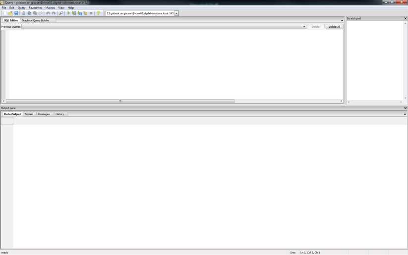
Figure 48: SQL Editor

Type your SQL statements in the top pane, and press F5 or click the green arrow to run your SQL. The results and messages will appear in the lower pane.

A side note on using SQL in Postgres

Using SQL in Postgres is likely to cause some users problems: Postgres is case sensitive by default. If you create a table or other object with a name with specific casing, it will create exactly that name. However, when trying to access the object, Postgres will look for the object name using all lowercase letters unless the name is enclosed in quotation marks.

As an example, if I CREATE TABLE Shawty, then the table will be named Shawty with a capital S. But if I then run SELECT * FROM Shawty, Postgres will fail to find the table. Instead, I need to type SELECT * FROM "Shawty" to make Postgres pay attention to the casing of the name.

This also extends to the Postgres data adapter for .NET. If you are unable to access a table in the Postgres data adapter, try putting the table name in quotation marks and you'll most likely find it resolves the issue.

Please note that regular strings are enclosed with single quotes, not double quotes. If you enclose your literal string in double quotes, Postgres will interpret your text as an object name and not as data.

The best practice for creating objects in Postgres is to give them all lowercase names. I've done exactly this for the database I'll be using to demonstrate the SQL functions, and I've changed all the names of tables and columns to lowercase after importing the data as shown previously. I've also removed columns from the dataset that are unused either in the examples, or in general.

If you receive errors while trying the samples, make sure that you're making the same changes I am, using single and double quotes properly, and correctly casing names as needed.

Testing the Output Functions

Let's try the following:

You should receive something like the following output:

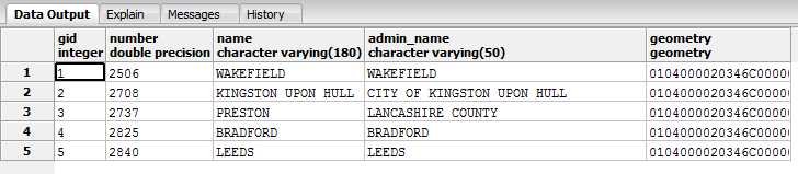
Figure 49: Data Output with Binary Geometry

As you can see, the geometry column is displayed in its binary form, which may or may not be in WKB format.

Now let's try this:

You should receive the following:

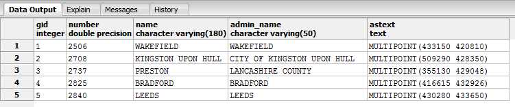
Figure 50: Data Output with Text Geometry

As shown in the previous figure, the output is in WKT format with the coordinates in meters since we're using OSGB36 as the SRID.

Let’s swap AsText for AsEWKT. We should get the following:

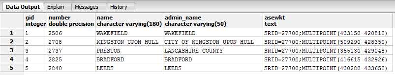
Figure 51: Data Output with EWKT Geometry

You may have noticed that in these examples I've been calling the functions without the ST_ in front. ST_ is a legacy tag from when systems were called Spatial and Temporal systems. In most modern GIS databases, you can freely switch between using the prefix and leaving it out since most systems define the function both with and without the 'ST_' prefix. One or two functions are defined only with the ST_ prefix, so if something seems to be missing in your data, try both spellings before you give up.

As you can see, the main difference between AsText and AsEWKT is the addition of the SRID in the output.

Let's try one more, this time with the data output in GeoJSON format:

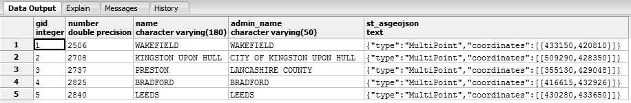
Figure 52: Data Output with GeoJSON Geometry

What Else Can We Do with Spatial SQL?

We can do tons of things with spatial SQL. A better question is what can't we do? However, as a developer, you're most likely only interested in simple tasks, so we'll continue by looking at a few real-world scenarios and what our database can do to help us.

Scenario 1: Largest land mass

Let's suppose you have a number of land plots for sale, and you have them all in a nice mapping system that potential buyers can browse via a map-enabled website. One thing you may want to know is which plot has the largest area so you can price them appropriately.

This is achieved very simply by using the area functions provided by the database.

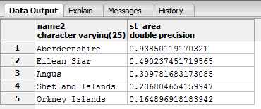
Figure 53: Calculated Land Areas

You'll notice that all our results are in square degrees or fractions thereof. This is because our geometry was added to the database in WGS84 (SRID 4326) coordinates. Most of the calculation functions will return their answers in the same units that the source geometry uses. Converting our area results to meters is not difficult.

SRID 27700, if you recall, is measured in meters so all we need to do is transform our geometry from SRID 4326 to SRID 27700. We can do this using ST_Transform.

The transform function takes the geometry to be transformed as the first parameter, and the SRID to transform it to as the second. Using the function on our data gives us the following SQL:

Figure 54: Geometry Converted from Square Degrees to Meters

Once you have the data converted from square degrees to meters, you can then use normal SQL order by clauses and other aggregate functions to arrange the areas from largest to smallest, or add a price column. For example, the following code outputs the five largest counties in the U.K. and their areas in square meters.

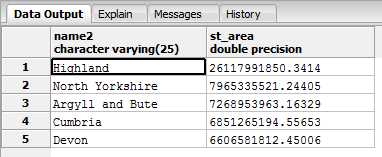
Figure 55: Five Largest Counties in the U.K in Descending Order

Another thing that might be useful to know is how long the perimeter of the land mass is. Finding this is just as easy, as shown in the following code sample and data output:

Figure 56: Perimeter of U.K. Counties

Scenario 2: How many of what are where?

Another typical use of GIS is for gathering information on how one object's location is related to another object's location. For example, given three U.K. counties—Durham, Tyne and Wear, and Cumbria—we can easily find out how many principal towns are in each.

This code gives us the following:

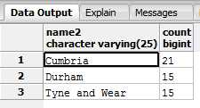
Figure 57: Number of Towns in Cumbria, Durham, and Tyne and Wear Counties

The SQL for this introduces the spatial function ST_Within, which tests to see if one geometry is fully within another.

There are two important concepts to remember from this example:

• For one object to be within another, the inner object must be fully inside the outer object's bounding line. In the county example, if your geometry is smaller than the thickness of any of the county boundary lines and lies directly on one, ST_Within would not have picked it up. Instead, it would have been identified as intersecting with the geometry rather than being within it.
• The order of parameters on some spatial SQL functions is important. In the county example, if you switch the order of the county and town parameters, you'll find that you receive no results because a point cannot fully contain a polygon that is much larger than itself.

Because spatial SQL accounts for boundary polygons when performing relationship-based measurements, there are a number of different functions that perform very similar tasks with slight differences.

In the case of ST_Within, we have the following similar functions:

• ST_Contains
• ST_Covers
• ST_CoveredBy
• ST_Intersects

The Postgres and OGC specifications document the differences in fine detail way better than I can describe here, but essentially one only works on the interior of the polygon, and the others work on combinations of the interior enclosing ring and various levels of intersection.

As a developer, you'll most likely never use anything other than ST_Within, and in rare cases ST_Contains, for most of the GIS work you'll do.

In our counties example, you can also see that we've had to use ST_Transform to transform our counties into the correct SRID again. If you keep all your geometry in the same SRID when loading your database, you begin to see how much simpler your SQL can be.

Scenario 3: How close is this to that?

Knowing how far away something is always has a place in GIS. Whether you need to know how close the nearest McDonald's is, or how close a friend's house is, this is one of the most common operations used in GIS since mobile phones started pumping locations out of a built-in GPS unit.

Not only can we get a measurement of the distance something is from the user, but a GIS database can also select objects based on distances from the user within bounding boxes and radii.

Let's try an example. Start by finding the distances of all the towns in County Durham from the principal city of Durham.

This code gives us the following:

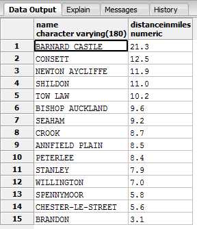
Figure 58: Distances of Towns from Durham in County Durham

The SQL we used is quite simple once you break it down. We performed a natural join on the towns and cities—both have exactly the same columns—on the admin name, using the admin name in the principal city as the master one. We filtered the cities so that only Durham is selected, and then we used ST_Distance(a,b) to get the straight line distance from geometry a to geometry b.

We then divided this distance by 1609.344 (the number of meters in a mile), cast the result back to a numeric (Output from ST functions are distance specific, e.g., meters, degrees, etc.), and rounded it to one decimal place, before ordering the towns from furthest to closest.

Brandon is the closest to Durham; Barnard Castle is the farthest away.

Now let's take a look at capturing items in a given radius. Again, we'll use Durham city as our center point, and cast a radius of 10 miles around this point. Then we will list any town that falls in that radius, irrespective of its county.

Figure 59: Towns within 10 Miles of Durham

There are 14 towns within 10 miles of Durham city, and as you can see not all of them are in County Durham.

You can also rewrite the SQL with the ST_Dwithin(a,b,distance) function as follows:

The only thing different is the <= clause in the last part of the WHERE statement, so what changes? Not much, really. However, if you're using bounding boxes and buffers, you'll often get better results using ST_Distance with a <= operator.

Again, we used the cast operator to make sure our data output a normal numeric type and rounded it to one decimal place, divided it by 1609.344 to convert it to miles, and finally filtered things so that only towns around Durham were included.

It's easy enough to exchange the Durham city geometry for a GPS point from a GPS device, for example, and list the towns around that point.

Or if your GPS is WGS84 (SRID 4326), you'll need to transform it to meters and OSGB36 (SRID 27700).

Scenario 4: What is my geometry made of?

In some cases you may need to take your geometry apart and reassemble it in a different way, or make a new geometry based on the original one.

First off, let's find out how many points make up the border around County Durham.

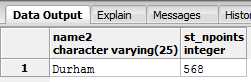
Figure 60: Number of Border Points

Or we can find the geographic center point of the county in the same coordinates as the actual geometry.

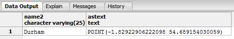
Figure 61: Geographic Center of County Durham

Or we can output a summary of what the object is.

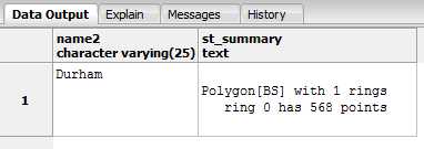
Figure 62: Summary of County Durham Object

We can also break down the underlying geometry. There are functions to dump entire sets of points that make up a boundary.

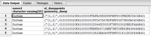
Figure 63: County Durham Boundary Points

Or we can get a specific point if the input is a LINESTRING or MULTILINESTRING.

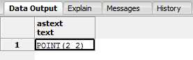
Figure 64: Finding a Specific Point

The point output shown in the previous figure is the second point in our linestring.

If you need to know the bounding box of an object, you can easily get the x, y pairs of the maximum and minimum extents by using the following code:

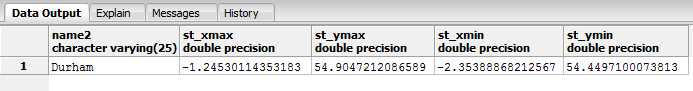
Figure 65: Maximum and Minimum Extents

Or if we need to perform measurements and other functions on our extents, we can get them as an actual geometric rectangle.

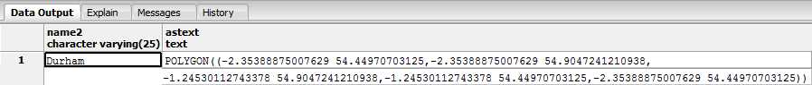
Figure 66: Extents Output as Geometric Rectangle

Lastly, let's imagine we have a segment of a path, represented by the following line:

Now let's try to make a new polygon based on a border around that line that is 5 units away.

This code gives us the following result:

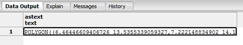
Figure 67: New Polygon Based on Line Segment Border

The output is a polygon with its center line exactly following our line, but 5 units away on all sides.

It's impossible to give examples of every possible scenario and combination in which you can use these spatial functions.  The main PostGIS reference can be found at http://postgis.org/docs/reference.html. I encourage you to spend time exploring them and trying the many examples given in the documentation, all of which should be possible using nothing more than pgAdmin's SQL editor.