Loading Data into Your Database

---

The first thing we need to do before we can begin to explore what a GIS can do is load some data in.

In this chapter, I'm going to load three ESRI shapefiles into Postgres to use with the demos later on. The first two of these will be point-based files showing the location of cities and towns in the U.K. The third file will be a polygon file showing the outlines of all the county and borough boundaries that make up the U.K.

For those of you who are not familiar with U.K. geography, the county boundaries logically divide the country into administrative regions, similar to the U.S. states or Chinese provinces.

Creating a Spatial Database

Before we can start to add any data into our system, we first need to create a database for storing the data. For the samples in this book, I'm going to create a simple three-table database rather than an entire GIS model as described earlier.

If you are working on a large enterprise application, I can't stress enough how important planning and design is in GIS database solutions. In many ways the planning part of this is substantially more important than the same steps in a normal database. Failures and alterations further down the line tend to be more pricey and more complex to fix for GIS solutions than for an average enterprise data solution.

To create the database, we'll be using the database admin tool provided with Postgres, pgAdmin. To start pgAdmin, click on the pgAdmin III icon on your desktop. If you don't see the icon, make sure that you installed the management tools when you installed the server.

Once you've installed the app and created an initial connection to your database server, you can start to create a database in that server connection as shown in the figures that follow.

Please note that for security reasons, I've removed server and table names from many of the figures showing pgAdmin in this book, leaving only those that are necessary for your understanding. In your use of pgAdmin, you'll see a lot more information when going through the steps I present here.

Figure 10: Creating a New Database

Right-click on the Databases item in your server tree and select New Database. This will launch the New Database dialog.

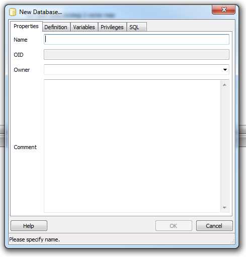
Figure 11: Naming the New Database

It's quite easy to see what needs to go where. All we need to do is give the database a name and an owner. You can fill in the Comment field if you wish; the rest you can generally leave with the default settings. Once you have the fields filled in, your dialog should look something like the following:

Figure 12: Completed New Database Dialog

Most Postgres installers create a template to aid in the creation of spatial database tables when using this or similar dialogs. Before we click OK, we need to navigate to the Definition tab and select the template to use as shown in the following figure:

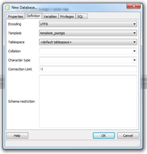
Figure 13: Choosing a Template from the Definition Tab

All the other options in this tab can be left as they are. Once you click OK, pgAdmin will return to the main display where you'll see your new database appear in the server tree.

Figure 14: New Database Added to Server Tree

It's also possible to create the database by hand using standard SQL commands such as Create Database and Create Table; however, using these can be a lengthy process.

There are scripts in the Postgres Contrib directory (located where you chose to install Postgres) that you can load and run to create all the spatial functions and metadata tables required. Since every installation of Postgres I've done has included pgAdmin, I've found it much easier and quicker to use the GUI. Please also note that even if you are installing your database on a platform such as Ubuntu, the pgAdmin tool can be downloaded separately from the Postgres website and installed on a standard Windows machine for managing your server.

Once the database has been created, you can expand the objects in the server tree to show the different tables and objects in your new spatial database.

Figure 15: Exploring the New Database

A Side Note about Postgres Users

Many of you reading this will likely be accustomed to using MS SQL Server for your data tasks. Postgres, like SQL Server, supports multiple user accounts. However, you need to be careful with using the root admin account.

In MS SQL, the super user account (usually sa) has ultimate control over the entire database. Under Postgres, the equivalent super user account is called Postgres, but unlike MS SQL, the Postgres user can be prevented from interacting with other tables.

If you create all your tables using the Postgres account you won't have an issue, but if you create databases and then assign ownership of these databases to other user names you have created in your server, you might find that the Postgres user account is unable to work with them.

This problem will most likely arise when opening database layers in QGIS. If you create a database connection using a given set of credentials, and create the database in pgAdmin using the Postgres user account, you'll find that the spatial metadata tables will have Postgres as their owner. When this happens, QGIS will be unable to open the metadata tables and will show no layers available for you to use in the application.

The solution to this is very simple. Using pgAdmin, right-click on one of the metadata tables and select the Properties option as shown in the following figure:

Figure 16: Editing Metadata Table Properties

The table's Properties dialog will appear.

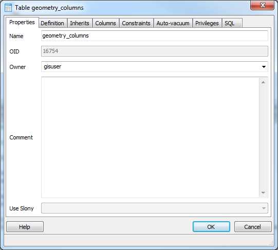
Figure 17: Editing the geometry_columns Table Properties

The Owner field provides a drop-down list of users defined in the server. Select the owner that you are using in your app connection.

Revisiting the Metadata Tables

If you remember from our discussion earlier in the book, we discussed the spatial metadata tables and the importance they have in the grand scheme of things.

If you've created your spatial database correctly, you should see two tables in your server tree: geometry_columns and spatial_sys_ref. Right-clicking on them and selecting View Data will allow you to examine what's in them as shown in the following figures.

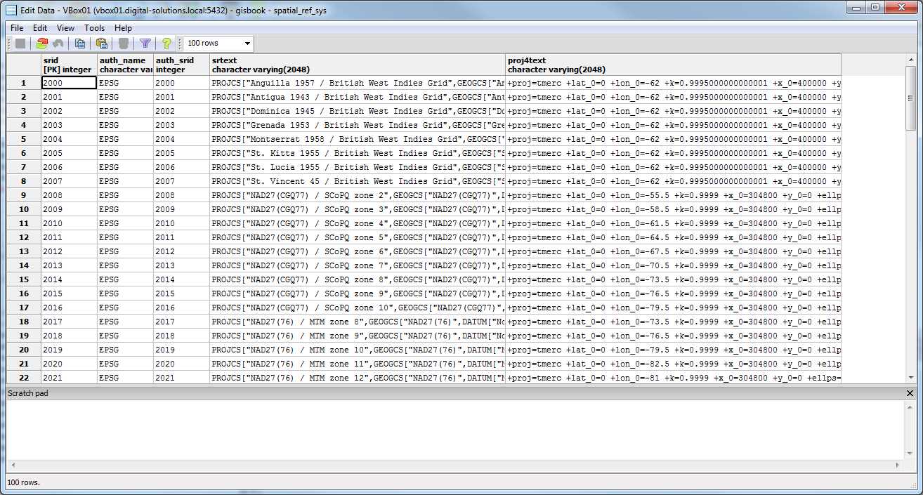
Figure 18: spatial_sys_ref Table

Figure 19: geometry_columns Table

As you can see, the geometry_columns table is initially empty. This will start to fill up as we load data into our database.

Loading Points Using QGIS

Quantum GIS has a great little tool built-in called SPIT (Shapefile to PostGIS Import Tool) whose sole purpose is to insert ESRI shapefiles into Postgres.

In practice, I have found that it gets upset easily if there's even the slightest bit of corruption or non-standard data in the shapefile you are trying to import. Despite its fragility, it remains the most used tool by QGIS users to import data into their database.

You activate SPIT by clicking the small blue elephant icon on your QGIS toolbar as shown in the following picture:

Figure 20: Activating SPIT

Once SPIT loads and displays its main interface, you should see the following:

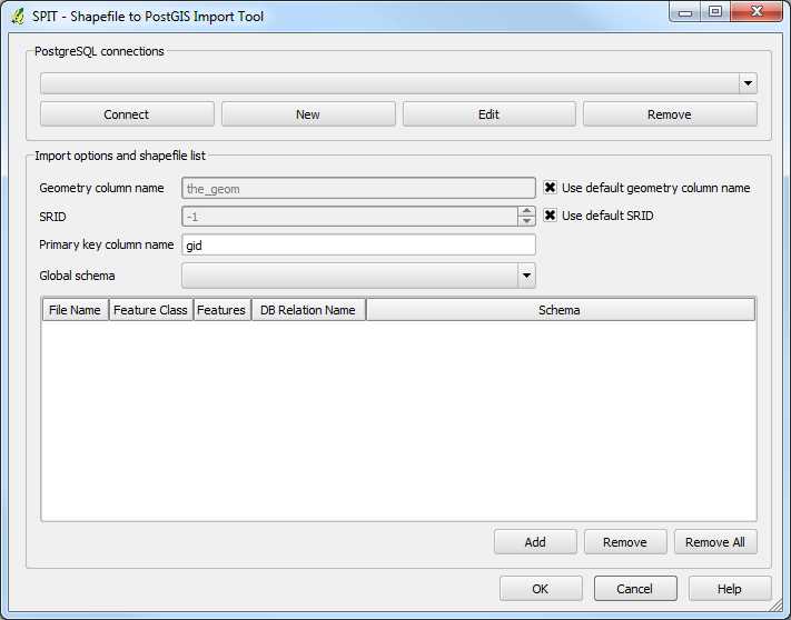
Figure 21: SPIT Interface

The interface is fairly self-explanatory. The PostgreSQL connections area is where you'll find any connections to your SQL databases listed. The Import options are for specifying things like the SRID of your data, and other options for the data import.

Your PostgreSQL connections list is shared between here and the main app. If you've already created a connection in QGIS, you'll be able to reuse it here by just selecting it from the drop-down and clicking Connect.

For the purposes of this exercise, however, we'll be creating a new connection to hold our data. To start, click New under PostgreSQL connections. The Create a New PostGIS connection dialog will appear.

Figure 22: Creating a New PostGIS Connection

Complete the fields as shown in Figure 22, remembering to substitute your server name, database name, user name, and password as required for your own Postgres installation.

You don't have to save the password and user name, but it makes connecting easier if you  don't have to type the credentials in every time.

The four deselected options are not required. They are used to control the following:

• Only look in the geometry_columns table: This option means exactly what it says. By default, QGIS will look at all tables in the database to see if any of them contain spatial geometry. Selecting this check box prevents this.
• Only look in public schema: If you use different schemas to logically divide your database, selecting this option will make QGIS only look in the public schema (equivalent to DBO in MS SQL).
• Also list tables with no geometry: Selecting this option will make QGIS list tables with no geographic data in the Add Layer dialog.
• Use estimated table metadata: If you have a table that is not registered in the geometry_columns table, selecting this option will make QGIS guess the data type, rather than examine the data in the table to determine the geometry type.

Once the fields are completed, click the Test Connect button. The test should be successful.

Click OK to save the connection and register it in the SPIT tool.

Once you return to the SPIT dialog, click Connect, and then use the Add button to browse and load the shapefiles for U.K. towns and cities.

You can download sample shapefiles from bitbucket.org/syncfusion/gis-succinctly.

Once you've set the other options such as the SRID—all files provided for these demos are in UK-OSGB36, SRID 27700—and the Geometry column name, your SPIT dialog should look similar to the following figure:

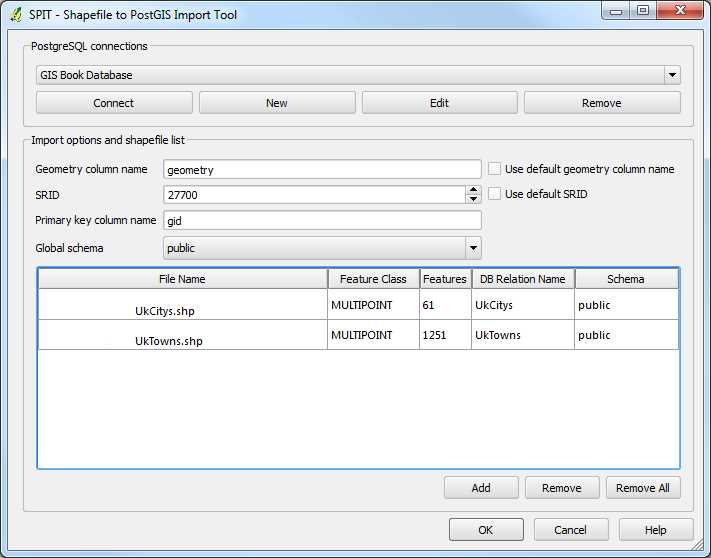
Figure 23: Completed SPIT Dialog

Click OK to add your data into your Postgres database and create any tables and other objects needed. If you go back to pgAdmin after adding your data and look at the geometry_columns table, you'll see that there are now two entries in it.

Once SPIT has finished, you should be able to go back to the main QGIS window and display a Postgres vector layer. We'll wait to do this for the moment though; next we're going to load the county boundary polygons using GeoKettle.

Loading Boundary Polygons Using GeoKettle

Sometimes you need a little bit more control over your data loading process. For instance, you may need to combine two files and make some transformations to your data before importing it into your database.

When you need to go beyond simple loading using SPIT, you need to use an ETL (Extract, Transform, and Load) tool such as GeoKettle. As mentioned previously, GeoKettle is a specialized ETL package that understands geospatial data and all its special metadata.

As with Postgres and QGIS, I'm not going to cover the installation process. It's fairly straightforward if you download the Java installer version. Since it requires Java to run, make sure you have an up-to-date Java VM installed on your computer.

After installing GeoKettle, open the program. You should be presented with something that looks like the following screenshot:

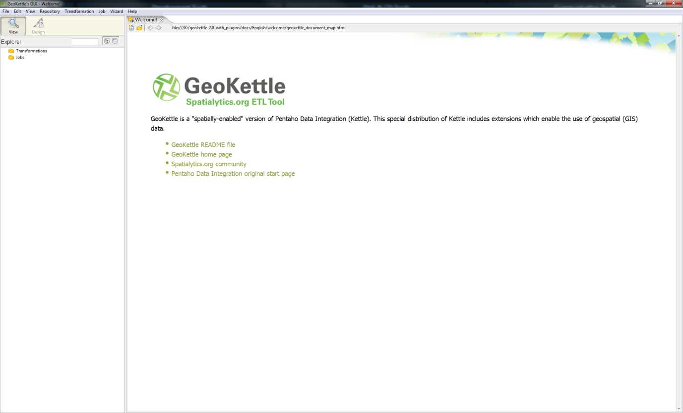
Figure 24: GeoKettle Home Screen

The concepts behind using GeoKettle are slightly different than the normal point-and-click methodology you may be familiar with, but once you get used to them working with GeoKettle is very easy.

Transformations and Jobs

If you click on the File menu and select New, you'll see that you have two options: Transformation and Job. The idea here is that many transformations make up a job, allowing you to break your task down into smaller chunks and then reassemble them using a sequence.

If you've ever done any workflow programming in .NET, you'll be familiar with the idea of separate work units and sequencing those pieces to perform a whole task. Using GeoKettle is the same idea. For what we are going to achieve here, we only need a simple transformation, so select the Transformation item under New.

Figure 25: GeoKettle File Menu

Adding Transformation Steps

Once you have a new GeoKettle work surface, you'll notice the designer palette in the left of your screen.

To construct a transformation, drag the necessary steps from this palette to your work surface, and then connect them together by holding Shift and dragging between them.

Data then flows from step to step in the direction of your connections, performing the required step as it passes through.

In order to add a shapefile to a database, we need three transformation steps:

1. A shapefile input.
2. A set SRID transform.
3. A table output.

Let's start by adding our input step. Select the Input folder in the design palette, and then drag a Shapefile File Input onto the work surface as shown in the following screenshot:

Figure 26: Adding a Shapefile Input Step to the Transformation

Open the Output folder in the designer palette and add Table output to the transformation.

Figure 27: Adding a Table Output Step to the Transformation

Open the Transform folder in the designer palette and add the Set SRS step.

Figure 28: Adding a Set SRS Step to the Transformation

Note the black arrow in Figure 28 pointing at SRS Transformation—be careful not to use this one as it is an actual data transformation. You may find that you need this if you're transforming your data from one spatial system to another; for example, if you have a GPS course recorded from a GPS device, it may be in WGS84 coordinate space, but you may need to change it to a local UTM system that matches your area of the globe.

Set SRS does NOT transform the actual coordinate values; it simply sets the SRID of the data you're adding. You must ensure that this SRID is the correct value; otherwise, when you try to demonstrate or project your data, your geometry will appear in a completely different place than where you expect it.

Once you've added the necessary steps to the workspace, you need to connect them. To do this, click on one of your steps to select it, hold Shift, and then click and drag to the step you wish to connect. One thing that may be confusing is that GeoKettle does not draw a line as you drag the pointer from one step to the next. Just keep moving the pointer to your next transformation step and release the mouse button when you reach it.

For our example, connect the Shapefile File Input to Set SRS, and then connect Set SRS to Table output. If all goes as expected, you should see something like the following:

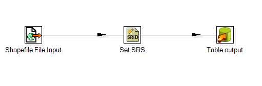
Figure 29: Connected Transformation Steps

Configuring the Steps

Once you have everything connected, you should be ready to configure everything. We'll start by configuring the shapefile input. Double-click the Shapefile File Input step to gain access to its properties.

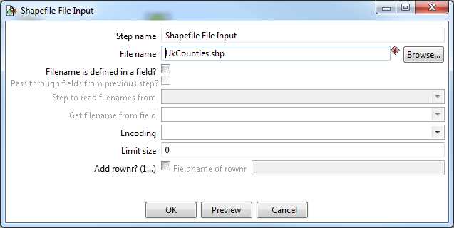
Figure 30: Configuring the Shapefile Input

The only thing we need to change is the file name. Click the Browse button, browse to the location of the sample shapefile for the U.K. county boundaries you downloaded, and click OK.

You can use the Preview button to take a quick peek at your file before you click OK. After clicking Preview, you'll be prompted for how many rows you want to preview.

Figure 31: Previewing the Shapefile Input

Entering 0 will show all the rows in the input file. Click OK to display the preview. GeoKettle will open the file and show you a spreadsheet-like view of the data and any attributes within the file.

Figure 32: Shapefile Data Preview—Standard View

You can click the Geographic view tab at the top to see the following:

Figure 33: Shapefile Data Preview—Geographic View

When you're finished previewing the data, click Close. Click OK in the Shapefile File Input dialog to complete the shapefile input setup.

The next thing we need to do is set our SRS options. In our case, as you may have noticed when previewing the data, our county boundaries shapefile is actually in WGS84 (SRID 4326) coordinate space. As mentioned previously, we are not going to actually transform the coordinates for this sample data, but in a production system it's highly recommended that you match all your data in the same coordinate space. If I was doing this for a production system, I'd use the SRS Transformation step and actually change the coordinates to OSGB36 (SRID 27700). For this example, I'm keeping things as simple as possible.

If you want to try transforming your data, note that you'll need two Set SRS steps, one on each side of the SRS Transform step, to ensure you have the correct spatial ID going into and coming out of the transformation.

Moving on in our example, let's set the singular SRID we need for this data. Double-click the Set SRS step to open its dialog; you should see the following:

Figure 34: Configuring the Set SRS Step

For the Set SRS on field drop-down, select the correct field to set the geometry on. Usually it is called the_geom in a shapefile. In the EPSG Code field, select the correct spatial ID for the data. In our case, it will be SRID 4326 (WGS84). You can look through the drop-down list to get an idea of how many SRID coordinate spaces there are. Rather than looking through the entire drop-down list, you can simply type 4326.

Once you've set the SRID, click OK to confirm the SRS settings.

The final step is to set our Table output and associated database connection. Double-click the Table output step to open its configuration dialog as shown in the figure that follows. Note that I've already filled in the connection and target table details.

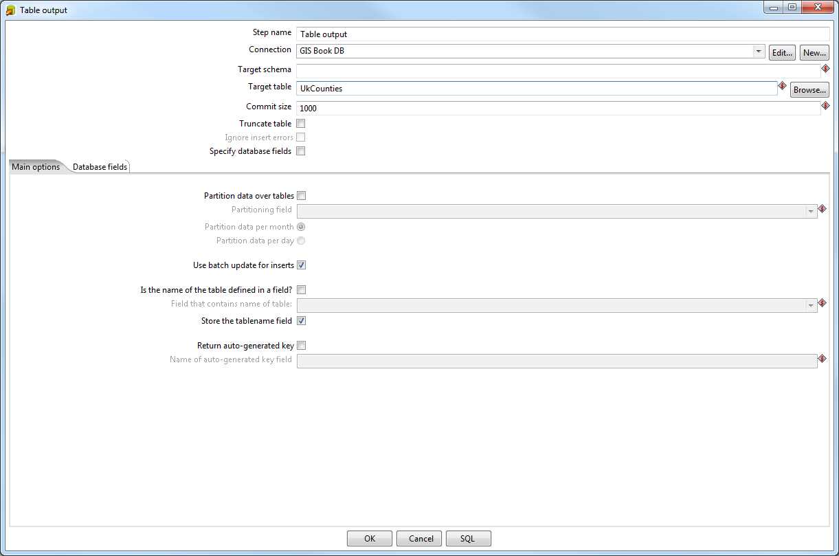
Figure 35: Table Output Configuration

The first thing you'll want to do is create a new database connection. Click the New button next to the Connection field. The Database Connection dialog will appear.

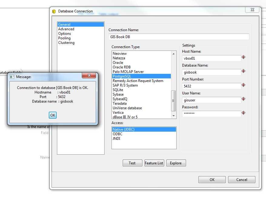
Figure 36: Adding a New Database Connection

Again for Figure 36, I've already filled in my details, but you should easily be able to see that GeoKettle supports a wide variety of database types.

Under Connection Type, select PostgreSQL. Under Access, select Native JDBC and fill in the appropriate details to connect to the same database you connected to when adding the point data using QGIS.

Once you’re done, give the connection a name and click the Test button. You should be shown a small dialog stating that the connection to the database is OK, as shown in the previous figure. Click OK to close the dialog, and click OK in the Database Connection window to go back to the Table Output options.

Next, you must set a target table name so the transformation step knows where to insert the data. You may also want to select the Truncate table check box to ensure the table is void of data before starting. The other table output settings can usually be left as they are.

If you’re creating the data for the first time, you'll need to click the SQL button at the bottom of the window to automatically generate and run the SQL necessary to create the initial table in your database. If you're using an existing table, this will give you the SQL needed to ensure the table schema matches the data. It's fairly straightforward, and if you have any knowledge of SQL you'll see immediately what's happening.

One thing I often do in the SQL dialog is add a primary key because GeoKettle does not automatically add one. There are transformation steps for adding primary keys and such, but I find it easier to add the extra field in the SQL editor when creating the table by manually typing in the extra line. In the following figure, you can see I added a primary key with the definition for GID in Postgres.

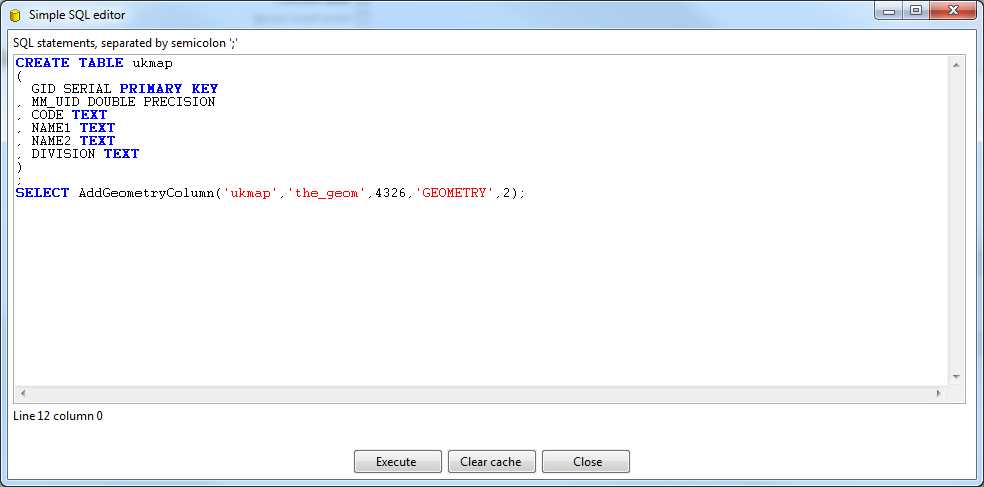
Figure 37: Adding a Primary Key

When you're done editing your SQL, click Execute to run it. Once you've run your SQL successfully, you can click Close to exit the SQL editor and then click OK to navigate back to the transformation workspace. You've completed setting up the required steps.

When you arrive at this point, go to File > Save to save your loading script. GeoKettle will refuse to run the transformation unless your file is saved. When your script is saved and you're ready to run the transformation, click the green play arrow in the toolbar.

Figure 38: Button to Run Transformation

The Execute a transformation window will appear.

Figure 39: Execute a Transformation Window

99 percent of the time you won't need to change anything in this window. Click the Launch button and the lower pane in your workspace will display the transformation progress.

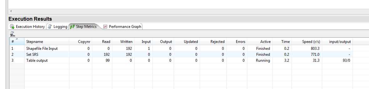
Figure 40: Viewing the Transformation Results

When all your Active column entries switch to Finished, you should have a database loaded with the county polygons; you are now ready to start experimenting.

If any of the steps turn red and display Stopped, you have a problem. The details and stack trace of the problem will be shown in the Logging and Execution History tabs. Unfortunately, as much as I'd like to be able to list every possible issue you'll see here, I simply can't. When GeoKettle fails, it only releases a stack trace and refuses to do anything further. This probably isn't an issue for the average developer, but for a non-technical user it can look very scary indeed.

My experience with transformation problems is that they're usually some kind of data format issue; for instance, an incorrect setting in the transform step of the destination server spitting out its default data because it doesn't like something about the SQL GeoKettle has just sent to it.

Whenever I receive a stop condition, I copy and paste the output from the Logging pane into a text editor so I can start examining SQL statements and diagnosing the stack trace in an easier-to-read window.

Once all of the transformation steps finish successfully, you can close GeoKettle and return to Quantum GIS. Using the connection you created when loading data with SPIT, you can view the data you now have in your database.

Previewing the Data

If we open Quantum GIS and start a new project, the first thing we need to do is set the project properties. We do this by navigating to Settings > Project Properties in the toolbar.

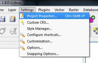
Figure 41: Opening Project Properties in Quantum GIS

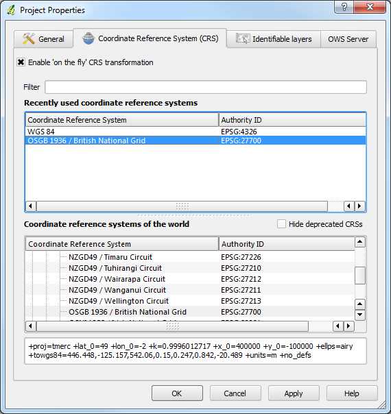
Figure 42: Quantum GIS Project Properties

In Project Properties, select the Enable 'on the fly' CRS transformation check box since we have both SRID 27700 and SRID 4326 coordinate systems in our database. As you can see in Figure 42, I've selected OSGB36 (SRID 27700) for my project since I reside in the U.K. You can choose WGS84 for your project if you want. As mentioned previously, it's a good practice to select a coordinate system specific to your location.

Once you've selected your coordinate system, click OK to return to the main Quantum GIS workspace.

Now we need to start adding vector layers from our database. Click the blue Add Database Layer icon on your toolbar. You'll be presented with the Add layers dialog, and should immediately recognize the Connections drop-down at the top of the dialog; it looks just like the one you used in SPIT.

Figure 43: Add Database Layer Icon

Figure 44: Adding Database Layers

Select the connection you wish to use from the drop-down, or create a new one as you did in SPIT, and click Connect. A list of vector layers present in your Postgres database should appear as shown in the following figure:

Figure 45: Available Vector Layers

As you can see, the two point layers we imported earlier and the polygon layer we imported using GeoKettle are available. Select all of them and click Add.

After a bit of processing, depending on your computer and database speed, QGIS should display the layers, hopefully in three different styles.

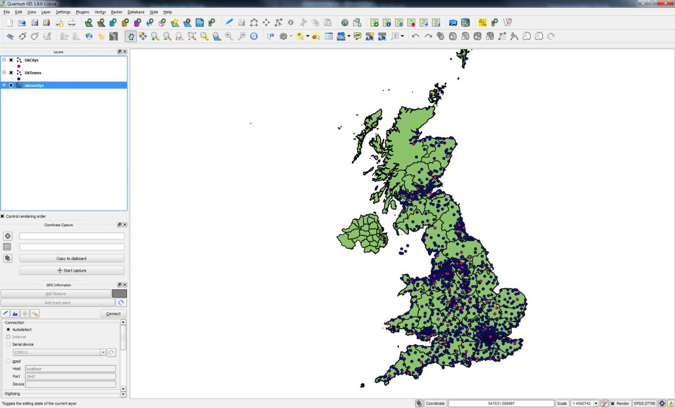
Figure 46: Loaded Map with Three Layers

As shown in my example in Figure 46, county boundaries are in green, towns are dark blue, and cities are pink.

If your display looks anything like mine, then congratulations, you've just created your very first spatially enabled database. Now we get to play with this data.