Physical Data Model

---

The physical model takes the logical model and defines items like the database tables, fields, and indexes necessary to store the entities of the model in a particular database management system. Typically, a database developer or database administrator should build the physical model since they likely are familiar with the nuances of the target database.

Tables

A table is a collection of fields that represent attributes from the logical model. Typically, the table will contain a primary key (PK), a way to uniquely identify each object in the table. The logical model attribute can be a single field, or a collection of fields, which together form the PK attribute. The primary key can be one or more columns, as needed to identify each record uniquely. Your logical model should indicate how the primary key is constructed.

Naming

There are few conventions for naming tables, although people are often opinionated about them. If your team has table naming conventions, you should adhere to them. If there are no naming conventions, consider defining them. A few suggestions follow.

Use singular form

This is a matter of preference, and other developers might suggestion plural table names. I like singular form because I find the syntax: Customer.Address clearer than Customers.Address. A table implies a collection of objects, so the plural form is somewhat redundant. Also, particularly in English, plural forms are not consistent. Customer becomes Customers, but Person becomes People, Activity become Activities, and Data remains Data.

Avoid database keywords

One convention that most developers agree on is not to use database keywords as table names. SQL Server for example, requires delimiters (brackets []) around table names that are keywords. mySQL uses backticks (`) around reserved words. There is no need to place a burden on anyone referencing the table to (a.) know the keywords, and (b.) know what delimiter should be used.

Be consistent with naming

If you have tables with similar content, try to keep the names similar. Calling the vendor table Vendor_location, and the customer table Customer_Shipping_Address is not a good idea if both tables contain address information associated with a company (vendor or customer).

Fields

The field is the smallest unit in the database, and all attributes will become one or more fields in the table. Each field will have a unique name within the table, a data type (with an optional size value), and an indication of whether the field can be empty (NULL value).

When defining a field, you should adhere to a few guidelines:

• Keep the field name the same across tables. If you decide to use POSTAL_CODE, don’t use ZIP or ZIPCODE in another table. 
• Select the smallest appropriate data type for the field.
• Always define NULL or NOT NULL, even if the database provides a default.
• Try to use CONSTRAINTS and DEFAULT values to ensure the quality of the data in the table.

When a database system retrieves a record, it copies the record into a memory buffer. The smaller the total record size, the more records can be placed into a buffer. If a query returns more than one record (likely), then the less memory needed for all the records, the better the performance will be. Also, many database systems will hold records in a cache, anticipating the records might be needed again. The more records that can be retrieved from the cache rather than by accessing the disk, the faster the query will perform.

Data types

There are four major data type categories that can be used in a SQL table. These are string, numeric, date/time, and Boolean (bit) value. Within each category, there typically are more detailed variations, such as size, range of dates, integer versus decimal, and so on.

In this section, we will describe Microsoft SQL Server data types. Appendix A lists the data types for other SQL versions (Oracle, mySQL).

String data types

The string types are referred to as CHAR data. The general syntax to define a character/string field is the following.

FieldName      CHAR (size) NULL | NOT NULL

When defining a string type, there are a few considerations. 

The CHAR(size) is a fixed size, it will always consist of the specified size characters. If the data content is shorter than the size, it will be padded out (typically with spaces).

The VARCHAR(size) is a variable sized string field, with a maximum of size characters.

If your field will always be the same size (such as two-character United States state code), CHAR data should be used. If, however, the content placed in the field varies substantially, you should use the VARCHAR data type. The VARCHAR data type places a bit more work on the server, since it needs to store an integer indicating how much data is in the field.

Note: In Microsoft SQL Server, the size parameter is optional, but if not provided, it defaults to 1. However, if you use CAST or CONVERT and don’t specify a size parameter, the default size is 30.

If you try to put more content than the size supports, you will receive an error message to the effect that data will be truncated, and the field will not be updated. Also, if an application code (say C#) retrieves the data from CHAR data, it will not be trimmed and might contain trailing spaces. If the application retrieves data from VARCHAR, it will be not have trailing spaces.

When deciding between CHAR and VARCHAR, you need to consider the tradeoffs. Since SQL knows the size of CHAR fields, it is easier to move them into a memory buffer. With a VARCHAR field, SQL needs to determine the size first, before adding it to the memory buffer. Using VARCHAR fields makes sense for many applications because the performance hit is measured in milliseconds. If you are consistently returning many records and performance is a top consideration, a CHAR field might be better.

The keyword MAX can be used in place of a size value, and typically would be used when fields vary greatly and could possibly exceed 8,000 characters. 

Unicode characters

The CHAR data typically holds ASCII characters, which are characters that can be represented by a single 8-bit value (1-256). However, if you are dealing with international data, it is possible that the data will be in Unicode (two bytes are needed to represent each character). If you anticipate UNICODE data, you can use NCHAR() or NVARCHAR(). In SQL Server, the LEN() function will return the number of characters in the field, while the DataLength() function will return the actual number of bytes used to hold the content.

Collation

In a simple world, all data could be stored in ASCII, and the numeric bytes would correspond to the same letter or symbol. However, SQL is used worldwide, and different countries and cultures use different alphabets and symbols. SQL lets you specify the set of characters and symbols (called a collation) to use. You can specify the collation at a server level, a database level, and even an individual field level.

To add a specific collation on a column, you simply add the keyword COLLATE, followed by the collation name. For example, the following.

Notes NVARCHAR(max) COLLATE SQL_Latin1_General_CP1254_CI_AS

This syntax would allow the notes to be entered using Turkish characters. In addition, the sort order is determined by the collation. The collation provides details, for example, of how to sort the Turkish characters ç, ü, and û.

You can find the collations on your server using the SQL command.

SELECT * FROM sys.fn_helpcollations()

WHERE name LIKE 'SQL%'

The following command will show you the collation of the server and database.

SELECT 'SERVER' as type,

        CONVERT (varchar(256), SERVERPROPERTY('collation')) as Collation 

UNION

SELECT 'DATABASE',

        CONVERT (varchar(256), DATABASEPROPERTYEX(db_name(),'collation'));

When to use character types

A character data type imposes the least restrictions on the type of data that can be entered, so you should keep that in mind when choosing the type. Some developers will simply use CHAR types for all fields, which is particularly common for date values. However, often a direct result of using CHAR fields for dates is getting an error message when trying to convert the string to a date. In SQL Server, the syntax IsDate(‘2021’) returns 1 (true), and will refer to 1/1/2021. If you anticipate doing any kind of operation on the field (such as adding days), you should use a better data type than CHAR data.

Numeric types

For numeric types, there are integer values and decimal values. The integer values are always exact values, and the type of integer (TINY, BIG, and so on) simply refers to the range of values that can be placed in the field:

• Bit: A Bit field can be 0, 1 or NULL (this is often used in place of the Boolean data type that SQL does not support).
• TinyInt: A whole number between 0 and 255.
• SmallInt: A whole number between -32,768 and 32,767.
• Int: A whole number between -2,147,483,648 and 2,147,483,647.
• BigInt: Whole number between -9,223,372,036,854,775,808 and 9,223,372,036,854,775,807.

Note: TinyInt does not allow negative numbers; you will receive an overflow message if you try to place a negative number into a TinyInt. (Similarly, you’d receive the same error message if you tried to set an integer value outside the allowed range.)

Working with integer data is generally quicker than decimal values.  

Decimal (numeric)

The decimal or numeric data type (they are functionally synonyms) are exact decimal values.  You will need to specify the precision (total number of digits) and the scale (digits to the right of the decimal points). The maximum precision is 38 digits, and the default precision is 18 digits.

The scale portion can be zero up to the precision specified. You cannot specify the scale without also specifying the precision.

If you try to place a number larger than the precision into the field, you will get an overflow error message. If you try to place a larger number into the scale, it will be rounded up or down.

Table 12 shows example values using a field with a Decimal (5,2) data type.

Table 12: Example numeric storage

Float and real

Floating point numbers are approximate values, which use less storage space than decimal values but don’t provide precise values. The floating data type specifies the size of the mantissa (which defines the number of bits to store). The mantissa value specified can be any number from 1 to 53, although SQL only uses 24 or 53 (numbers less than or equal to 24 are assigned size 24, and any number above that is assigned 53).

A double precision float (Float(53)) can hold 1.8 * 10³⁰⁸ (which is a lot of zeros). The real data type is a synonym for Float(24). If you are concerned with storage space, consider using a floating-point number, but be aware of the loss of precision that can occur.

Money types

SQL Server has two money types: smallmoney and money. The money types are accurate to a ten-thousandth of the monetary units. A period is used to separate the fraction (like cents) from the whole value (like dollars). The money data type can be many different currencies that support whole and fractional units, such as U.S. dollars, British pounds, or Japanese yen.

The smallmoney type can range between -214,748.3648 and 214,748.3647. The money data type can range between -922,337,203,685,477.5808 and 922,337,203,685,477.5807. money requires 8 bytes; smallmoney requires 4 bytes of storage.

Note that money types are based on INT and BIGINT, but the types support the decimal place splitting between whole and fractional currency units.

Date and time

SQL Server provides several different date and time data types, depending on the date range needed, when to include time, and the time zone offset:

• Date: The Date type holds only date values (no time portion) between 1/1/0001 and 12/31/9999. It is accurate to a single day, and defaults to 1/1/1900.
• DateTime: The DateTime type holds date values between 1/1/1753 and 12/31/9999 and includes a time portion between 00:00:00 and 23:59:59:997. It defaults to midnight, January 1 of 1900.
• DateTime2: This type is very similar to DateTime, with a wider range of dates (1/1/0001 through 12/31/9999) and more precise time (00:00:00 through 23:59:59:99999999).
• SmallDateTime: This is a version of date-time that uses less storage by only supporting dates of 1/1/1900 through 6/6/2079 and time down to the second (23:59:59).
• Time: Just the time portion with a range of 00:00:00:00000000 to 23:59:59:99999999.
• DatetimeOffset: This is just like DateTime2 (1/1/0001 through 12/31/9999), with the addition of the time zone offset (number of hours different from UTC time).

If you plan on any date manipulation, use the date and time data types.  A very common question on programming support boards deals with dates being stored in characters fields.

Boolean

SQL Server does not provide a Boolean data type, but the numeric BIT type can hold a 0, 1, or NULL. You could define a column as a BIT field, NOT NULL, to create a true Boolean value.

Constraints

A constraint can be added to the field definition, and this will control the type of data allowed in the field. Each database will have its own allowed constraints, but four common constraints are the following.

Primary key

The column (or columns) that forms the table’s primary key. By design, this column must contain unique values, since a primary key is the way to uniquely identify a row. Attempting to duplicate a primary key value will result in an error. In addition, a primary key cannot be NULL.

You can specify a primary key by adding the PRIMARY KEY keyword after the column definition.

ID int NOT NULL PRIMARY KEY

Alternately, you can do it by creating the constraint after the columns are defined.

PRIMARY KEY (id)

You should use the CONSTRAINT syntax to create a primary key on more than a single column, for example, ORDER_NO and LINE_ITEM_NO.

Foreign key

The column in the table must be NULL or match another table’s primary key. This is how table relationships are built. To create the foreign key, you will need to know the table and primary key column for the relationship.

To create the foreign key on the column definition, you can use the foreign key syntax.

LocationID int FOREIGN KEY REFERENCES ShippingLocations(LocationID)

You can create the foreign key after the columns are defined (which is necessary if more than one column is the key) using the FOREIGN KEY constraint syntax.

FOREIGN KEY (CustNo, LocaNo) REFERENCES Shipping(CustNo,LocaNo)

The reference should specify a table and its primary key (one or more columns).

Unique constraint

The unique constraint requires unique values for a column or columns within the table. If you are using a surrogate primary key (for internal storage) and a visible key for the user, be sure to add the unique constraint for the visible key.

A unique constraint can also be applied to a combination of fields. For example, we might want a constraint that user ID and email together must be unique. This would prevent a user from creating multiple accounts with the same user ID and a single email address.

You can add the keyword UNIQUE after a column definition to specify the column is unique.

If you need a unique set of columns, you will need to use the UNIQUE constraint, as shown in the following example.

UNIQUE (UserId, EmailAddress)

If you place the UNIQUE keyword after each field, you will require that each field individually must be unique, not the combination of the two fields.

Check constraint

A check constraint is a logical expression that must return TRUE for the value to be allowed in the column. For example, you might want to create a constraint that the due date of an invoice is not in the past.

Check (Inv_Due_Date >= GetDate())

Developers sometimes skimp on constraints, which can likely cause problems down the road.  For example, if a secondary key is used to identity the record (such as customer ID when the primary key is the customer record number), any code that references the customer ID probably expects a single row to be returned. If a unique constraint was not added and a customer ID gets duplicated, it will very likely break the code that never anticipated duplicate customer IDs.

Similarly, imagine a birth date field that allows future dates. What will the application code do when it computes a negative age for a person?

It is generally a good practice to constrain the data to prevent unexpected errors in the future.

Defaults

Defaults are field values that get placed into record if the field is NULL during an INSERT operation. Defaults only apply during an INSERT command. If your INSERT statement provides a value for the column, the default will not be used.

A default can be a constant (text or numeric value) or an expression that returns a constant value. You can also use some SQL variables, such as @@ServerName, and functions, such as db_name() or getDate(). getDate() is often used to default a column to the current date.

The DEFAULT keyword, followed by the value, can be specified on any column for which you wish to add a default value.

Note: DEFAULT only applies if you don’t specify the column name during the INSERT. If you specify the column name and pass it a NULL, the NULL value will be written to the column, not the DEFAULT value.

Computed fields

A computed column is a virtual column where the expression to compute the value is stored in the table, not the actual value.

To create the column, you provide a column name, the keyword AS, and a SQL expression. Whatever data type the expression returns will be the data type of the column. For example, the following syntax would return the total value of an inventory item based on quantity on hand and per unit cost.

Total_Value AS QtyOnHand * PerUnitCost

While this is a simple example, and could be computed in a front-end, if the formula was complex and used in multiple places, having the definition in the database can make sure the value is consistent across applications accessing it.

Note: Computed columns that are complex can slow down query performance, since the expression needs to be evaluated for every row. SQL Server allows you to add a PERSISTED option to the definition, meaning the value is saved when the row is INSERTED. It will be updated if the data is changed, but when just querying the data, the current persisted value will be shown, not recomputed.

Logical entities to physical table

For an example, let’s consider the customer entity, which we normalized in the prior chapter.  The logical model is duplicated in Figure 19.

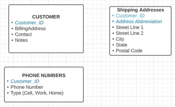
Figure 19: Customer logical model

Customer table

For the customer table, we need to select a primary key. There are a few different approaches we can use.  

Customer ID

We can create an identity column and use this as the key. The customer will never see the key, but it will be used to link the table together. This approach allows the system to maintain the key and prevent duplicate key values.

Tip: Often, a website might accept parameters to display customer information. If the parameter is an integer, a hacker might simply modify the URL and change the customer ID parameter, possibly viewing other customer data. Keep this in mind if you use a predictable pattern to assign ID values.

Another approach is like the identity column, but uses a GUID (globally unique identifier) as a primary key (using the NewId() function as a default for the Customer ID column). This will prevent hackers from viewing other records but will be less convenient as a parameter to a web URL.

We can create a key based on the customer’s name so the customer can easily remember the key. While this will make the key easier to understand, it also would be updated if the customer’s name changes.

For our customer table from the model, we are going to use the identity column for the key to link tables together and provide a different identifier for the customer to use.

Our final table design might look like this.

Table 13: Customer table

We defined the internal customer_ID to be an identity, surrogate key, and the CustomerCode to be the customer visible code for their company. We also require Postal_Code to be either five characters long or 10 (if company uses zip+4). Note that this example only considers addresses in the United States.

The Notes field is set to varchar(max), which allows unlimited notes to be added. However, the notes are assumed to be English or other European languages. If we want to allow foreign text, we can use the nvarchar() data type instead.

Figure 20 shows the SQL Server transact-SQL code to create the table.

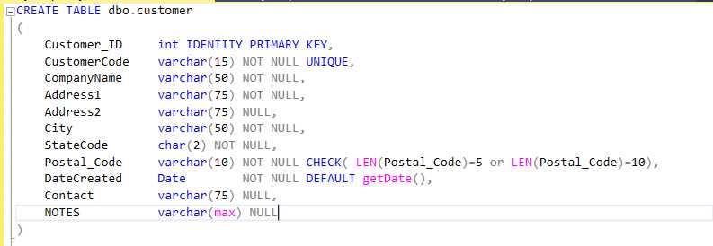
Figure 20: Create customer table

SQL Server provides certain extended properties about the column in the table. A useful property is a column description field. You can add customer descriptions to a table using the sp_AddExtendedProperty stored procedure. For example, Figure 21 shows how to add a description property to the CustomerCode for this table.

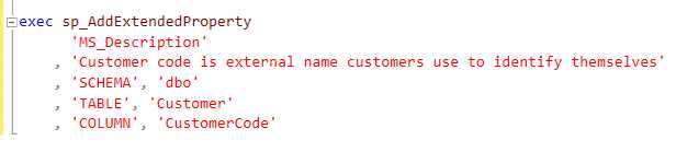
Figure 21: Add Description property

Since the MS_Description property is not standard, you will need to use the system tables to get the description. Code Listing 1 shows the code to display the column name, type, and description for a table.

Code Listing 1: Show column properties

The Description property can be a handy documentation component when building your database, and it will be maintained within the database for future reference. You can also set a table-level property by not providing a column name in the stored procedure.

Address table

The address table is used to provide the alternate shipping locations that a customer might have. The table design might look like this.

Table 14: Address table

We would add the following constraints to this table.

PRIMARY KEY (Customer_ID,AddrAbbr)

FOREIGN KEY (Customer_ID) REFERENCES Customer(Customer_ID)

When we create the order table, we will have a foreign key relationship to the address table, so the warehouse knows to which address to ship the products and the preferred shipper to use.

Figure 22 shows the code to create the shipping address table.

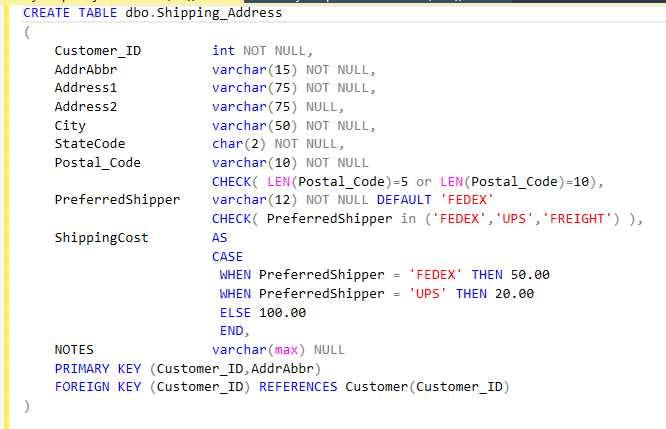
Figure 22: Create shipping address table

After a few descriptions and running the query in Code Listing 1, we can see the table details in Table 15.

Table 15: Documentation for shipping address table

Phone number table

The phone number table is simply a list of phone numbers and types associated with the customer. As currently described, it is simply a list of phone numbers within a key to identify individual phone numbers. While this logical design is technically accurate, I would suggest we always add a primary key (surrogate key in this case). 

With this tweak, our phone number table could look like this.

Table 16: Phone number table

The reason I suggest the surrogate key is to make the rows easier to update and delete. In addition, at some future point, you will likely be asked to be able to identify a particular phone number from the list.

Figure 23 shows the code to create the phone numbers table.

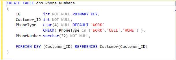
Figure 23: Create phone numbers table

Indexes

SQL can create an index to improve performance of the statement to retrieve data. An index is like a book index, a keyword or keywords, and a record number where it can be found. Imagine a phone book (an ancient book containing an alphabetical list of names and phone numbers). You would likely open the book to the middle and see what letter the names begin with (then either open the book to another page higher or lower until you find the name). This is a binary search, which is a very simplified explanation of how indexes work.

SQL will create indexes on primary keys automatically, but you can decide what other indexes would be useful. In our phone book example, imagine you need to find a phone number, but you only know the street name. Starting at page one and looking for the street would be very slow (in SQL, this is called a table scan). Creating an index on the street name (keyword and page) would allow you to find the phone number by street name much quicker.

While SQL will allow you to create any number of indexes (subject to database limits), there is a performance cost when adding to or editing the database, since the index likely needs to be updated, as well. You need to consider your queries and consider adding indexes for the very commonly looked up fields. In our customer table, the CUSTOMER_ID field will automatically have an index, since it is the primary key. You might want to add a second index on the customer code, since that is most likely how the various departments will look up the customer information.

With SQL Server and other database systems, you can often profile your queries to pick up suggested indexes if a query is running slow. The syntax to create an index is the following.

CREATE INDEX <name> ON <table (field or fields)>

We could create the customer code index as follows.

CREATE INDEX byCustCode ON Customer(CustomerCode)

Determining which indexes to create is often a matter of trial and error to improve query performance. Very small tables (lookup tables) often only need the primary key index. Large, user-facing tables generally have multiple indexes based on the end users’ use of the system.

Views

One of the minor drawbacks of data normalization is that some simple queries become more complex when you need to join tables together. For example, if our employee table supports multiple phone numbers for employees, and we wanted an internal phone number list, our query could look like the following snippet.

SELECT emp.first_name,emp.last_name,

       IsNull(pho.PhoneNumber,’<none>’ as WorkPhone

FROM employee emp

LEFT JOIN phone_numbers pho on pho.EmployeeId=emp.ID and Phonetype=’WORK’

A person who is less familiar with SQL might not understand that query, so we can create a view to make it simpler to reference the phone list.

CREATE VIEW work_phone_list

AS

SELECT emp.first_name,emp.last_name,

            IsNull(pho.PhoneNumber,’<none>’ as WorkPhone

FROM employee emp

LEFT JOIN phone_numbers pho on pho.EmployeeId=emp.ID

          AND Phonetype=’WORK’

Now the user simply can write the following.

SELECT * FROM work_phone_list

The complexity of the JOIN query is hidden from the user. We can also use this approach to return only a subset of fields. If an employee record included salary information, we might want to create a view for Human Resources that only returns columns other than salary information.

Note: Views cannot include an ORDER BY clause in most database systems, although there are ways to work around it, depending on the SQL system used.

Summary

We provided a high-level overview of how to create a physical model in this chapter using Microsoft SQL Server. Every database package has its own enhancements and nuances, possibly additional field types, table features, and so on. Once you have the general table and field definitions spelled out, you can work with the database administrators to best create your tables using the best features from the database package.