NVIDIA Visual Profiler (NVVP)

We will now shift our attention to something completely different. We will step away from straight CUDA C coding and look at some of the other tools, which collectively form the CUDA toolkit. One of the most powerful tools that comes with the CUDA toolkit is the NVIDIA Visual Profiler, or NVVP. It offers a huge collection of profiling tools specifically aimed at drilling down into kernels and gathering hundreds of interesting performance counters.

Using a profiler can greatly help code optimization and save programmers a lot of time and trial and error. NVVP can pinpoint many possible areas where the device could potentially be used more efficiently. It runs the application, collecting thousands of metrics from the device while the kernel executes. It presents the information in an effective and easy-to-understand manner.

Older devices with compute capability 1.x do not collect the same metrics as newer devices. If you are using an older device, you may find that the profiler has insufficient data for some of the following tests. The profiler will not generate the charts depicted in the figures when there is no data.

Starting the Profiler

The visual profiler will be installed to any one of several different locations, depending on the version of the CUDA Toolkit you have installed. The simplest way to run the profiler is to search your installed apps for NVVP. You can search for NVVP using the Start menu for Windows 7 and previous versions, or the Start screen in Windows 8.

When you run the NVVP application, you will see a brief splash screen. Then, you should see the main profiler window. A wizard may open and assist you in creating the project and loading a program to profile.

To open a program for profiling, open the File menu and choose New Session. You will see the Create New Session dialog. I will use the shared memory version of the nearest neighbor algorithm (from Chapter 7) for testing out the profiler in the following screenshots, but you can load any .exe file here. Type a path to an .exe file you have compiled or find the compiled file you wish to profile by clicking the Browse button (see Figure 8.1). It is usually best to profile applications which are compiled with optimizations (i.e. release mode rather than debug). The performance difference between release mode and debug is vast, and the profiler’s information on a debug mode program is probably not relevant at all to the release mode compilation.

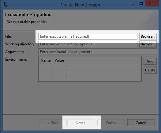
Figure 8.1: Create New Profiler Session

You can select the working directory and command line arguments to pass the program when it executes, as well as environment variables, if needed. The only setting that is required in the Create New Session dialog is the File setting. Once you have chosen the file, click Next.

The next page of the dialog allows you to specify some basic profiling settings, like whether the application should be profiled straight away (or if the profiler should simply locate the file and await your command to begin the profiling) and what the device's driver timeout should be. Click Finish to create the profiler project. If you left the Start execution with profiling check box selected, the program will run and profile your application straight away.

Tip: Use the Generate Line Number Info option in Visual Studio to get the most out of the visual profiler. The profiler is able to provide detailed information when the compiled program includes line number references. This option can be set to Yes (-lineinfo) in the Project Settings dialog in Visual Studio, in the CUDA C/C++ section.

General Layout

The profiler consists of a menu bar and a toolbar at the top of the window, and three subwindows, each containing one or more tabs (see Figure 8.2). The top-left window provides an overview of the kernels and other CUDA API function calls. It consists of a collapsible tree view of devices (including the host), streams, and contexts that are active in the application.

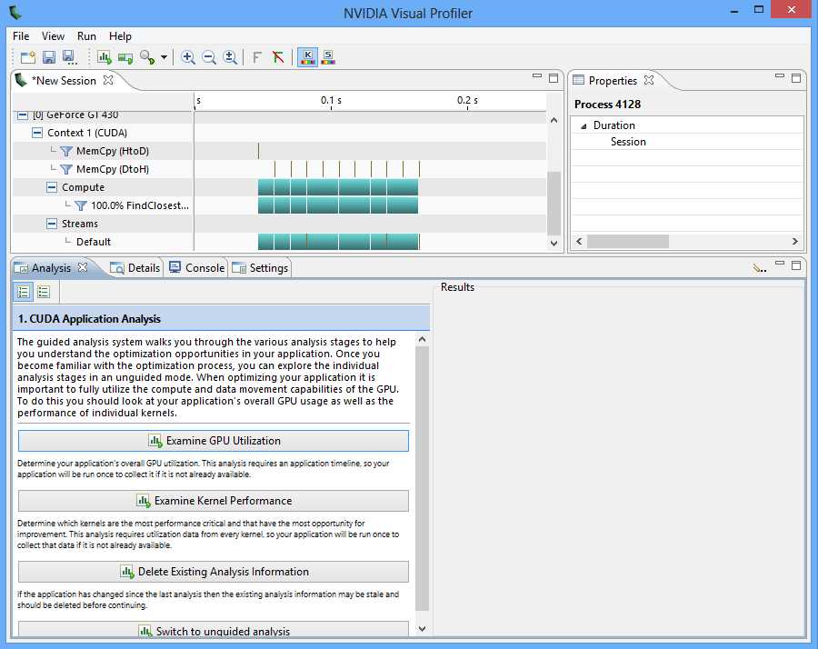
Figure 8.2: Main Window of NVVP

This overview panel also contains a chart to the left of the tree view. The rows of the chart can be opened or closed using the tree view. The chart depicts the amount of time taken for kernels to execute and the CUDA API function calls. The longer a function or kernel takes, the longer the bar representing the call will be.

If you choose not to profile the application straight away or need to re-run the profile after making changes to the .exe, you can click the Play button in the toolbar (the one with a loading bar behind it) to re-run the profile at any time.

Once the application has been profiled, select the bar that represents the kernel call you are interested in. I have selected the first call to FindClosestGPU in Figure 8.3.

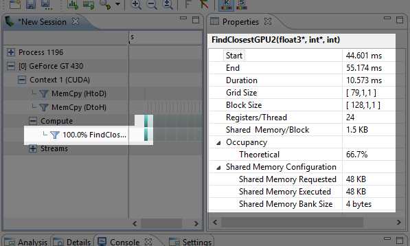
Figure 8.3: Properties of a Kernel Call

The Properties panel will be filled with information about the kernel call (right side of Figure 8.3). The start, end, and total execution time is displayed in milliseconds. The launch configuration shows that the grid consisted of a total of 79 blocks, each with 128 threads.

There are metrics for register counts per thread and shared memory per block. We will examine these in more detail shortly because they greatly influence the occupancy metric. The next number is theoretical occupancy. We will also examine occupancy in detail as we progress through this chapter, because of the generated achieved occupancy metric, which tells us the actual occupancy a kernel achieved, not just the highest theoretical occupancy.

The final three properties show the amount of shared memory the SMs requested, how much they were given, and the word size of the banks of shared memory (which is 4 for all current cards).

Occupancy

Occupancy is a simple metric for determining how busy the device is compared to how busy it could be. Occupancy is the ratio of the number of concurrently running warps divided by the maximum number of warps that could be running with the particular device.

Concurrent warps may or may not actually run at the same time. A warp is said to be active (concurrently running) if the device has allocated the resources (shared memory and registers) for the warp. The device will keep a warp active until it has finished executing the kernel. It will switch back and forth between active warps in an attempt to hide the latency of memory and arithmetic caused by the warps as they execute instructions.

Usually, the more warps running concurrently (the higher the occupancy), the better the utilization of the device, and the higher the performance. If there are many warps running concurrently, when one is delayed, the scheduler can switch to some other warp and thus hide this delay or latency.

Tip: The CUDA Toolkit supplies an Excel worksheet called the CUDA Occupancy Calculator. This can be found at C:\Program Files\NVIDIA GPU Computing Toolkit\CUDA\v6.5\tools or a similar folder, depending on your installation. The worksheet allows you to quickly input the compute capability, shared memory usage, register counts per thread, and block size. It calculates the theoretical occupancy and shows detailed charts depicting the possible outcome of varying the block size, the register counts, the shared memory usage, or all three. Figure 8.4 shows screenshot of the calculator.

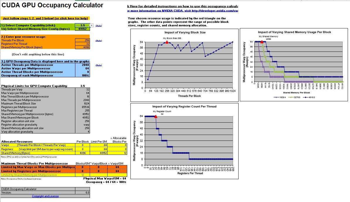
Figure 8.4: CUDA GPU Occupancy Calculator

The maximum number of threads per SM (according to the output Device Query for my device; be sure to check the output for your own hardware) is 1,536 (or 48 × 32). This means for 100 percent occupancy, the kernel would need to have a total of 1,536 threads active at any one time; anything less than this is not 100 percent occupancy. There is most likely more than one SM in the device (again, according to Device Query for my hardware there are two), and the total number of active threads is 1,536 multiplied by the number of SMs in the device. For instance, if there are two SMs, the total number of active threads could potentially be 3,072.

This maximum occupancy can only be achieved with very special care. The number of threads per block, registers per thread, and shared memory per block work together to define the number of threads the SM is able to execute concurrently.

Note: Maximizing occupancy is not always the best option for optimizing a particular kernel, but it usually helps. For a very enlightening presentation on optimizing certain kernels with low occupancy, see Vasily Volkov's 2010 GPU Technology Conference (GTC) presentation, Better Performance at Lower Occupancy. The slides are available at http://www.cs.berkeley.edu/~volkov/volkov10-GTC.pdf. The presentation was recorded and is available online from GTC on demand at http://www.gputechconf.com/gtcnew/on-demand-gtc.php.

Register Count

Each SM in the device is able to execute up to eight blocks concurrently, and up to 48 warps, but only if resources permit. One of the governing resources is the register count per thread. The Register/Thread metric in Figure 8.3 shows how many registers are used per thread. The number of registers used is related to the number of variables (and the variable types—for instance, doubles take two registers each) in the kernel's code. Reusing a small collection of variables in the code rather than defining many different variables will generally decrease the number of registers per thread, but usually at the expense of code complexity.

If this value is high (perhaps 40 or 60 registers per thread) and there are a considerable number of threads per block, the SMs will not be able to execute 48 warps concurrently.

Tip: NVCC can return verbose information. This output includes, among other things, a printout of the register usage per kernel to Visual Studio's output window during the project build. If you wish to enable this output, set the Verbose PTXAS Output option to Yes (--ptxas-options=-v) in your project's properties in the CUDA/Device section.

Note: There is a single additional, implicit register used per thread, which is not reported in the profiler or with the verbose PTXAS output. All register counts should have this additional register added to be accurate. Instead of a maximum of 64 registers per kernel, we are limited to 63.

The maximum number of concurrent threads per SM for this device (GT 430 according to Device Query) is 1,536 (48 warps of 32 threads each). The maximum number of registers (reported by Device Query) is 32,768, or 32k. If each thread uses 24 registers (plus a single implicit register), then 1,536 threads would use 25 × 1,536; or 38,400 registers. This number is greater than the 32,768 available registers, so the device cannot possibly perform at 100 percent occupancy. Each warp would require 32 × 25 (since there are 32 threads per warp) registers, or 800. The number of available registers divided by this value and rounded down will yield the approximate number of active warps an SM can execute, 32,768 / 800 = 40. This means the number of active warps the device could execute if it had only a single SM would be 40 instead of the maximum of 48.

Tip: There is a very simple way to reduce the register usage of threads—set the MaxRegCount value in the project's properties. In the CUDA C/C++ tab under the Device subheading, one of the options is labeled Max Used Register. Set a small number here if your kernel's register usage is limiting occupancy. Be careful! Do not set this to an impractically low value (such as 1 or 2); your code may take a very long time to compile or not compile at all. A setting of 0 (default) means NVCC will decide how many registers to use. Setting values lower than the number NVCC would use will generally mean that local memory is used when registers spill, and may not give you any extra benefit in increasing performance.

Shared Memory Usage

The total amount of shared memory on the device is 64k, of which some portion will be used as L1 cache. The kernel in this example used 16k of L1 cache and 48k of shared memory. Each block used an array of float3 structures, which has a sizeof value of 12 bytes each. There were 128 elements in the array, so the total shared memory usage per block for this kernel is 128 × 3 × 4 bytes, which is 1.5 kilobytes.

The SM will execute up to eight blocks at once if resources permit. Since 48k / 1.5k = 32, our shared memory usage would actually permit 32 simultaneous blocks. This means that shared memory is not a limiting factor on the occupancy for this kernel.

Unguided Analysis

We can get a lot more detail from the profiler by selecting a particular instance of the kernel in the graphical display window and using the unguided analysis option. In the following screenshot (Figure 8.5), I have selected the first kernel launch.

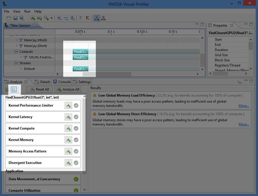
Figure 8.5: Unguided Analysis

Clicking the Run Analysis buttons (these are the buttons with a small chart and green arrow in the Analysis tab of the left panel) will re-run the application in the profiler, but it will collect the specifically requested data on the currently selected kernel. The selected kernel will usually take much longer to run because the profiler collects information as it executes the code.

Kernel Performance Limiter

The information from an unguided analysis can help you pinpoint exactly where the bottlenecks in your code are. Clicking on the Kernel Performance Limiter button in this example produces the following chart (Figure 8.6).

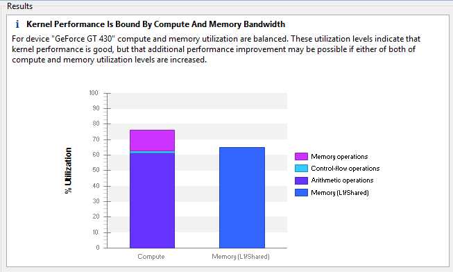
Figure 8.6: Kernel Performance Limiter

Control flow and memory operations are only a small portion of the Compute bar in Figure 8.6. The Memory bar shows that we are relying heavily on shared memory and not using the L1 cache at all. This heavy use of shared memory was intentional; it is the result of the blocking technique we applied in Chapter 7.

The arithmetic operations portion of the Compute bar is glaringly large. The chart indicates that if the kernel is to execute much faster, it will require much less arithmetic. To decrease the amount of arithmetic in a kernel, we would need to either simplify the expressions (which will probably not offer a substantial gain since the expressions were not complicated), or we can use a more efficient algorithm.

Our algorithm, which is essentially just a brute force linear search, was a poor choice. Each point is compared to every other point in the entire array, and if we really wanted to reduce the amount of arithmetic, we would investigate storing our points in a more sophisticated structure where we wouldn’t need to perform so many comparisons. The profiler has not directly said this, but it can be gleaned from Figure 8.6. Our kernel requires too many point comparisons, and that is the main reason it is slow.

Kernel Latency

The Kernel Latency option produces a sophisticated output of charts that indicate what might be limiting the occupancy of the kernel (see Figure 8.7).

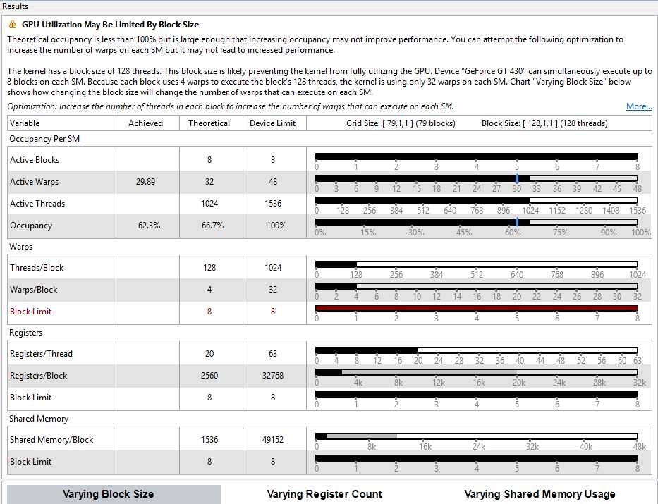
Figure 8.7: Kernel Latency

This option also produces the achieved occupancy statistic in the Properties tab, just above the theoretical occupancy. The output in Figure 8.7 compares the achieved occupancy with the maximum. It indicates quite clearly that the block size (128 threads) is a possible limiting factor.

For this particular kernel and this particular device, this tip from the profiler makes little to no difference on overall performance. I tested many block sizes and found that although larger block sizes increase the occupancy (for instance, 512 threads per block achieves an occupancy of 92.2 percent), the overall performance remains the same. The suggestion from the profiler to increase the block size is, in this instance, not beneficial, but this will often not be the case.

Kernel Compute

When we use the Kernel Compute option, we can see again that arithmetic is probably a bottleneck in our code. The chart in Figure 8.8 (the output from the Kernel Compute analysis) also shows that our texture compute usage is non-existent. Storing points as textures and allowing the texture units to perform at least some of the computation might improve our performance.

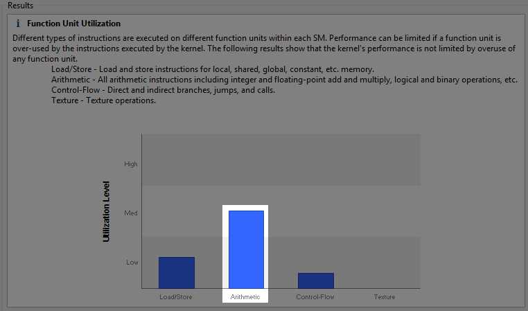
Figure 8.8: Kernel Compute

Kernel Memory

The Kernel Memory usage profile shows that our shared memory usage is unsurprisingly quite high from the blocking technique we employed in Chapter 7 (Figure 8.9). The texture cache reads are very low since we did not use any texture memory at all. This output again suggests that there may be some benefit gained if we can figure out a way to use texture memory for our current problem.

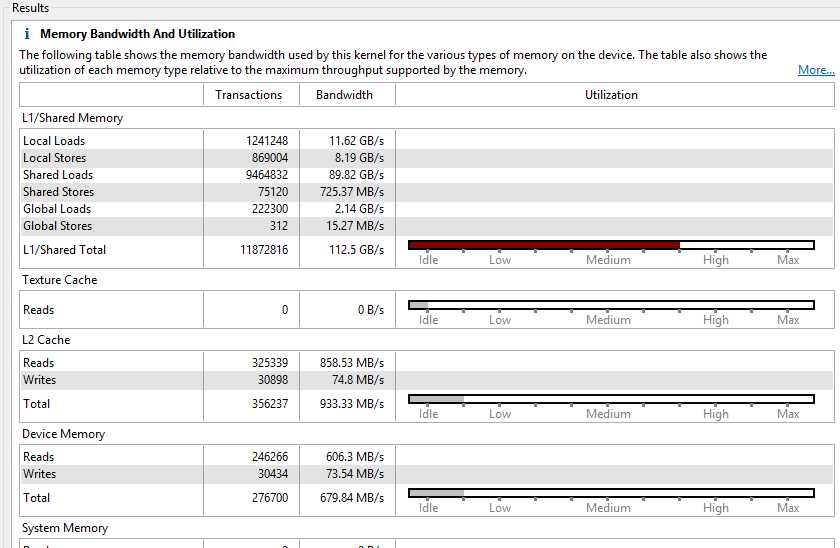
Figure 8.9: Kernel memory with shared memory blocking

The “Idle” readings for L2 and device memory are often a good thing since these memories are very slow compared to shared memory. Figure 8.10 shows the Kernel Memory usage profile for the original CUDA version of the algorithm (where we did not use shared memory). I have included it as it makes for an interesting comparison.

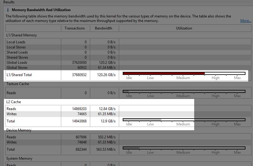
Figure 8.10: Kernel memory without shared memory blocking

The difference in performance (from 37 milliseconds in our Chapter 5 algorithm to 12 milliseconds in our Chapter 7 algorithm) is almost entirely attributed to the L2 cache being employed in the original code. The original version of the code (which leads to Figure 8.9) used L1 cache extensively. When the original kernel’s code executed, points were evicted from L1 to L2 when they were actually going to be read again in the very near future. The difference between the use of L2 and shared memory blocking gave us the healthy 300 percent performance gain.

Data copied to the device using cudaMemcpy always goes through the L2. In Figure 8.8, the L2 reads are showing that the points were read from L2 into our shared memory blocks.

Memory Access Pattern

To perform memory access oattern unguided analysis, you must generate line numbers when you compile your application. This option will examine the efficiency of the usage of global memory. Figure 8.11 is an example output.

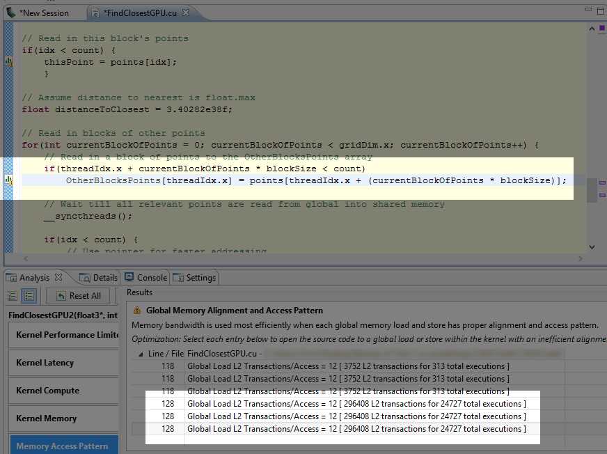
Figure 8.11: Memory Access Pattern

The top three lines (those referencing line 118 in the code) are potentially not as important as the lower three. Line 118 is where we read a single point from global memory into each thread. There are three transactions here because the structure (float3) is made of three floats. The following three transactions are potentially much more important to us (they reference line 128 in the code where we read global memory into blocks of shared memory). It is clear from Figure 8.11 and knowing how our blocking worked that the transaction counts at line 118 (3,752) are completely insignificant compared to the line 128 transactions (296,408) seen further down. If we needed to optimize based on this output, we should start by looking at line 128 rather than line 118.

In this particular code, you can see that this point is not making any difference whatsoever on the actual performance of the kernel. If we comment out line 128 in the code and re-run the kernel, it achieves exactly the same performance.

In the original CUDA version of the algorithm (from Chapter 5), the inner loop was causing 37,520,000 transactions (not shown in the screenshot). In the new version (from Chapter 7), the global memory transactions of the inner loop are completely negligible and not shown by the profiler at all in Figure 8.10. What we are looking at instead is the comparatively tiny number of transactions involved in creating the shared memory blocks. The 296,408 transactions from reading the blocks into shared memory are a vast improvement over 37,520,000.

Divergent Execution

The final option (second to last if you are using CUDA version 6.0 or higher) in the unguided analysis is the divergent execution analysis. In our particular kernel the divergence of threads within a warp is irrelevant and the threads of each warp act in lockstep almost all of the time. This type of execution pattern is ideal for CUDA and it is possible here because our algorithm was embarrassingly parallel. There is almost no communication required between threads whatsoever (except for the occasional block-wide barriers __syncthreads()).

Thread divergence is a tricky problem to solve. A good way to think about solving poor performance from thread divergence is to alter the data, the algorithm, or both instead of trying to optimize small sections and maintaining the same algorithm, data structure, or both. Minimize thread communication and synchronization. Organize data such that large groups of consecutive threads (i.e. 32 threads of a warp) will most likely take the same branches in an if statement.

Tip: When questioning how data might be better be stored and accessed, consider Array of Structures versus Structure of Arrays. Known as “AoS vs. SoA,” this concept involves a perpendicular rotation of data in memory to improve access patterns. For example, instead of storing 3-D points as [x₁, y₁, z₁, x₂, y₂, z₂...], the data is stored with all the x values first, followed by the y and then the z, e.g., [x₁, x₂, x₃..., y₁, y₂, y₃... z₁, z₂, z₃]. In other words, instead of storing data as an array of points (AoS), it might help access patterns to store three arrays—one for the X values, one for the Y values, and one for the Z values (SoA).

Tip: CUDA can be used to perform one algorithm quickly, but it can also be used to perform the same algorithm multiple times. This seemingly obvious statement is always worth considering when deciding what should be converted to CUDA. For instance, in a string search, we could use CUDA to search quickly for a particular sequence of characters. But a completely different approach would be to use CUDA to simultaneously perform many searches.

Other Tools

Details Tab

The Details tab gives a summary of all kernel launches. This information is essentially the same as the information in the Properties window, but it is given for all launches at once in a spreadsheet-like format.

Tip: If you have a kernel selected in the graphical view, the details will be displayed for that kernel only. To show all details, right-click in the graphical view and select Don't Focus Timeline from the context menu.

Metrics and Events

Finally, from the Run option in the menu bar, you can select to collect or configure metrics and events. This will open a window that allows you to specify the exact statistics you are interested in collecting (see Figure 8.12).

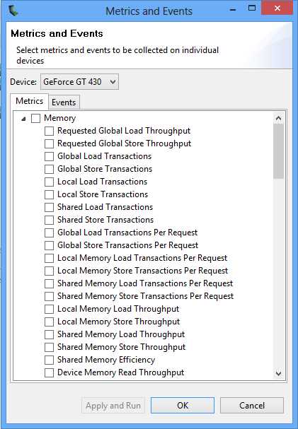
Figure 8.12: Metrics and Events

The benefit of specifically defining the metrics you are interested in is that when you click Apply and Run, the metrics will be collected for all the kernels. In the previous sections, the data was collected for the selected kernel alone. The output metrics are not shown in the Properties window but the Details panel.

In addition to this, you can select many metrics at once by selecting the root nodes in the tree view (Figure 8.12). This allows you to quickly select all metrics and run a gigantic analysis, collecting information on every aspect of every kernel in an application. It takes some time to complete the analysis, depending on the kernel. The output from such a request is a proverbial gold mine for studying possible optimizations. The entire Details panel can be exported to a comma separated values (CSV) file and opened in a standard spreadsheet application. To export the Details panel, click the Export Details in CSV Format button in the top right of the panel (see Figure 8.13).

Figure 8.13: Export details to CSV format