Neural Network Classification

This chapter explains how to perform classification using CNTK. Take a look at Figure 4-1 to see where the chapter is headed. The problem is to predict the species of an iris flower (setosa, versicolor, or virginica) based on four predictor variables (sepal length, sepal width, petal length, and petal width). A sepal is a leaf-like structure.

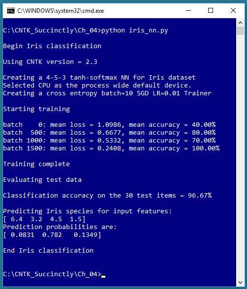
Figure 4-1: Iris Dataset Classification Using CNTK

Predicting a categorical value is often called classification, as opposed to predicting a numeric value, which is often called a regression problem. Note that logistic regression, explained in Chapter 2, is both a regression technique (the value to predict is a numeric probability between 0.0 and 1.0) and a classification technique (the prediction probability is mapped to one of two categorical values, such as “male” or “female”).

The example program creates a 4-5-3 neural network, that is, one with four input nodes (one for each predictor value), five hidden processing nodes (the number of hidden nodes must be determined by trial and error), and three output nodes (because there are three possible species). The neural network uses tanh activation in the hidden nodes and softmax activation in the output nodes.

The underlying error function used for training is cross-entropy, instead of the main alternative, squared error. The neural network is trained on 120 training items using the mini-batch approach, 10 training items at a time, and 2,000 iterations. During training, the average error/loss gradually decreases and the classification accuracy mostly increases, suggesting that training is working.

After training completed, the trained model was applied to 30 previously unseen test data items. The model scored 96.67% accuracy (29 of 30 correct predictions). The program concluded by using the trained model to predict the species for predictor values (6.4, 3.2, 4.5, 1.5). The predicted probabilities were (0.0831, 0.7820, 0.1349), which maps to (0, 1, 0), which is the encoding for the Iris versicolor species.

Preparing the Iris Data training and test files

Fisher’s Iris Data, created in the 1930s, is arguably the most well-known dataset in machine learning. There are 150 data items. The raw data looks like the following:

5.1  3.5  1.4  0.2  setosa
4.9  3.0  1.4  0.2  setosa
. . .
7.0  3.2  4.7  1.4  versicolor
6.4  3.2  4.5  1.5  versicolor
. . .
6.3  3.3  6.0  2.5  virginica
5.8  2.7  5.1  1.9  virginica

The first four values on each line are sepal length, sepal width, petal length, and petal width. The last value on each line is the species. There are 50 of items each of the three species. The example program uses data in a format that can be used efficiently by CNTK. That data looks like the following:

|attribs 5.1 3.5 1.4 0.2 |species 1 0 0
|attribs 4.9 3.0 1.4 0.2 |species 1 0 0
. . .
|attribs 7.0 3.2 4.7 1.4 |species 0 1 0
|attribs 6.4 3.2 4.5 1.5 |species 0 1 0
. . .
|attribs 6.3 3.3 6.0 2.5 |species 0 0 1
|attribs 5.8 2.7 5.1 1.9 |species 0 0 1

The |attribs and |species tags mark the start of the feature values and the class label values, respectively. Each line is space-delimited. The feature values don’t need to be normalized because they’re all roughly in the same magnitude. The species label is 1-of-N (also called one-hot) encoded.

You can use whatever tag names you wish. And you can add item ID numbers or comments using the tag mechanism, for example:

|ID 001 |attribs 5.1 3.5 1.4 0.2 |species 1 0 0 |# setosa
|ID 002 |attribs 4.9 3.0 1.4 0.2 |species 1 0 0 |#
. . .
|ID 041 |attribs 7.0 3.2 4.7 1.4 |species 0 1 0 |# versicolor
. . .

The 150-item dataset was split into a 120-item training set (the first 40 of each species) and a 30-item hold-out test set (the remaining 10 of each species). The CNTK-format training and test data can be found in the Appendix to this e-book.

Because there are four features, it’s not feasible to graph the data. However, you can get a rough idea of the data’s structure by examining the two-dimensional graph, based on just sepal length and petal length, shown in Figure 4-2.

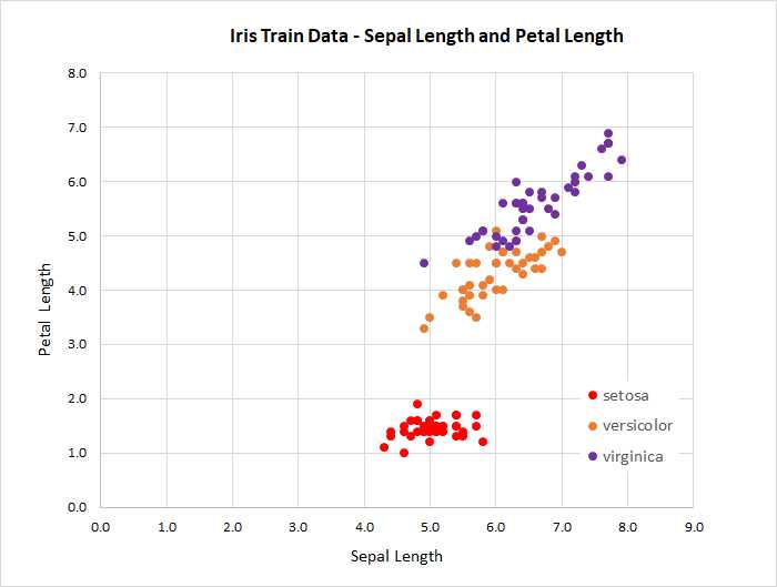
Figure 4-2: Iris Data

The classification program

The code for the program that generated the output shown in Figure 4-1 is presented in Code Listing 4-1. The program begins by defining a create_reader() helper function that can process data files in CNTK format:

def create_reader(path, input_dim, output_dim, rnd_order, sweeps):
  # rnd_order -> usually True for training
  # sweeps -> usually C.io.INFINITELY_REPEAT for training OR 1 for eval
  x_strm = C.io.StreamDef(field='attribs', shape=input_dim, is_sparse=False)
  y_strm = C.io.StreamDef(field='species', shape=output_dim, is_sparse=False)
  streams = C.io.StreamDefs(x_src=x_strm, y_src=y_strm)
  deserial = C.io.CTFDeserializer(path, streams)
  mb_src = C.io.MinibatchSource(deserial, randomize=rnd_order, max_sweeps=sweeps)
  return mb_src

There is a lot going on in the helper function, but for most classification problems you can think of the code as a boilerplate, and the only thing you’ll need to change is the references to the tag names in your CNTK file, attribs and species in this example.

Code Listing 4-1: Iris Flower Classification

Program execution begins by setting up the architecture arguments for the neural network, and the location of the data files:

def main():
  print("\nBegin Iris classification \n")
  print("Using CNTK version = " + str(C.__version__) + "\n")
  input_dim = 4
  hidden_dim = 5
  output_dim = 3
  train_file = ".\\Data\\iris_train_cntk.txt"
  test_file = ".\\Data\\iris_test_cntk.txt"
. . .

The dimensions for the neural network input nodes and output nodes are determined by the structure of your data, but the number of hidden nodes is a free parameter (often called a hyperparameter), and must be determined by trial and error. The data files are placed in a Data subdirectory. When working with CNTK, a standard approach is to have a root project directory for code, with Data and Models subdirectories.

Next, the classification program creates the untrained neural network:

  # 1. create network
  X = C.ops.input_variable(input_dim, np.float32)
  Y = C.ops.input_variable(output_dim, np.float32)

  print("Creating a 4-5-3 tanh-softmax NN for Iris dataset ")
  with C.layers.default_options(init=C.initializer.uniform(scale=0.01, seed=1)):
    hLayer = C.layers.Dense(hidden_dim, activation=C.ops.tanh,
      name='hidLayer')(X)
    oLayer = C.layers.Dense(output_dim, activation=None,
     name='outLayer')(hLayer)
  nnet = oLayer  # nnet = C.ops.alias(oLayer)
  model = C.ops.softmax(nnet)

The hidden layer nodes and the output layer nodes are created using the Dense() function, which fully connects all nodes in one layer to the other layer. The syntax is rather unusual. The X object, which is type CNTK Variable, acts as input to the hLayer object (the hidden layer), and the hLayer object acts as input to the oLayer object (the output layer).

The hidden layer uses tanh activation, which often (but not always) performs a bit better than the logistic sigmoid, C.ops.sigmoid() function. If you have experience with other deep learning libraries, you’ll likely be surprised that the output layer uses no activation function, or stated equivalently, uses the identity function. Many other deep learning libraries have a plain vanilla cross-entropy error function for training. Somewhat unusually, as of version 2.3, CNTK has a cross_entropy_with_softmax() function, but does not have a plain cross-entropy function. So, during training you must use cross_entropy_with_softmax() which expects raw, un-softmaxed values. If you apply softmax to the output layer, then during training softmax will be applied twice. This doesn’t break training, but for interesting technical reasons, double application of softmax often slows training significantly.

This explains why you don’t want to apply softmax to the output layer nodes. However, when it comes time to use the neural network, for evaluation or to make predictions, you typically want to apply softmax. So, the example program creates an nnet object, which is used during training, and a model object, which is used for evaluation or prediction.

The Python with statement is a shortcut that can be used to apply specified values to multiple layers of the network. In this case, the init parameter value means that all weights are initialized to a uniform random value between -0.01 and +0.01 inclusive. The example does not use the related init_bias parameter, so all biases are initialized to 0.0. Neural networks are often highly sensitive to initialization values, so if training fails, one of the first things to try is a different initialization algorithm. Some common alternatives to uniform() initialization are normal(), glorot_normal(), and glorot_uniform().

After creating the dual untrained models, the example program sets up a Learner algorithm object, and then uses it to create a Trainer training object:

   # 2. create learner and trainer
  print("Creating a cross-entropy batch=10 SGD LR=0.01 Trainer \n")
  tr_loss = C.cross_entropy_with_softmax(nnet, Y)  # not model!
  tr_clas = C.classification_error(nnet, Y)
  max_iter = 2000

  batch_size = 10
  learn_rate = 0.01
  learner = C.sgd(nnet.parameters, learn_rate)
  trainer = C.Trainer(nnet, (tr_loss, tr_clas), [learner])

As explained earlier, the nnet object, not the model object, is trained. The tr_loss object specifies cross-entropy error rather than the main alternative, squared error, for training. The tr_clas object is created so that classification error (percentage of incorrect predictions) can be automatically computed during training.

The learner object is a stochastic gradient descent object created using the sgd() function with a constant, fixed learning rate, which is the simplest possible algorithm. The CNTK library has a large number of sophisticated learning algorithms, many of which are very complex. For example, the using the CNTK fsadagrad() (“specialized adaptive gradient”) function, the learning algorithm could be coded as:

  max_iter = 2000
  batch_size = 10
  lr_schedule = C.learning_parameter_schedule_per_sample([(1000, 0.05), (1, 0.01)])
  mom_sch = C.momentum_schedule([(100, 0.99), (0, 0.95)], batch_size)
  learner = C.fsadagrad(nnet.parameters, lr=lr_schedule, momentum=mom_sch)
  trainer = C.Trainer(nnet, (tr_loss, tr_clas), [learner])

When advanced learner algorithms work, they can work very well. But you have many additional free parameters to deal with. As a general rule of thumb, I recommend that you try sgd() first, and resort to exotic learning algorithms only when you have a good reason to do so (such as repeated training failures, or known research results).

After creating the Trainer object, the example program calls the program-defined create_reader() function to create a Reader for the training data:

  # 3. create reader for train data
  rdr = create_reader(train_file, input_dim, output_dim,
    rnd_order=True, sweeps=C.io.INFINITELY_REPEAT)
  iris_input_map = {
    X : rdr.streams.x_src,
    Y : rdr.streams.y_src
  }

When training a neural network, you want to visit the training data in a random order so that the training doesn’t fall into some sort of oscillating pattern and stall. The sweeps parameter is set to the CNTK integer constant INFINITELY_REPEAT (18,446,744,073,709,551,615) so that training items can be visited multiple times.

The iris_input_map object is a dictionary collection, which is easy to botch. Notice that there are CNTK Variable objects (X and Y) on the left side of the colon, and assignment receivers from the call to the StreamDefs() function (x_src and y_src) on the right-hand side of the colon. As before, however, you can consider this code boilerplate, and just replace the map name (iris_input_map) with something pertinent to your classification problem.

Next, the example classification program trains the network like so:

  # 4. train
  print("Starting training \n")
  for i in range(0, max_iter):
    curr_batch = rdr.next_minibatch(batch_size, input_map=iris_input_map)
    trainer.train_minibatch(curr_batch)
    if i % 500 == 0:
      mcee = trainer.previous_minibatch_loss_average
      macc = (1.0 - trainer.previous_minibatch_evaluation_average) * 100
      print("batch %4d: mean loss = %0.4f, accuracy = %0.2f%% " \
        % (i, mcee, macc))
  print("\nTraining complete")

The next_minibatch() function fetches a batch of training items from the training data file (10 in this case), and knows where the feature values are, and where the class labels values are from the information supplied by the iris_input_map object. The call to train_minibatch() is almost too simple—all the real work was done in the preparation to the call.

It’s important to monitor the error/loss during training because training failure is very common, and so you want to catch it as early as possible. The example program displays the average cross-entropy error on the just-used mini-batch of 10 training items, and the classification accuracy of those 10 items, every 500 iterations/mini-batches. The CNTK library has a built-in ProgressPrinter class in the logging package. Many of my colleagues like and use a ProgressPrinter object, but I prefer to create logging messages using custom code.

After training using the 120-item training data has finished, the example program evaluates the classification accuracy of the trained model on the held-out 30-item test data:

  # 5. evaluate model using test data
  print("\nEvaluating test data \n")
  rdr = create_reader(test_file, input_dim, output_dim,
    rnd_order=False, sweeps=1)
  iris_input_map = {
    X : rdr.streams.x_src,
    Y : rdr.streams.y_src
  }
  num_test = 30
  all_test = rdr.next_minibatch(num_test, input_map=iris_input_map)
  acc = (1.0 - trainer.test_minibatch(all_test)) * 100
  print("Classification accuracy on the 30 test items = %0.2f%%" % acc)

The Reader for the test data specifies the location of the test data file and passes False to the rnd_order parameter because there’s no need to process the test data in a random order to determine classification accuracy. The sweeps parameter is set to 1 because you only want to visit each test item once.

The call to next_minibatch() will return all test items because the num_test variable is set to 30, the number of test items. The test_minibatch() function returns the classification error, which in my opinion isn’t quite as natural a metric as classification accuracy, so the example program computes accuracy from error, and prints the accuracy using a 0% to 100% format, in this case 96.67% (29 of 30 correct).

It’s sometimes useful to see exactly which data items were predicted correctly and incorrectly. You can walk through the test data and get detailed information like this:

  for i in range(0, num_test):
    curr_item = rdr.next_minibatch(1, input_map=iris_input_map)
    x = curr_item[X].asarray()[0]  # (1,4)
    y = curr_item[Y].asarray()[0]  # (1,3)
    p_prob = model.eval(x)  # prediction probabilities
    p_class = np.argmax(p_prob[0])  # predicted class 0, 1, or 2
    a_class = np.argmax(y)  # actual class 0, 1, or 2
    print(x, end="")
    if p_class == a_class:  # if predicted class == actual class
      print("  correct")
    else:
      print("  WRONG")

The code is a bit trickier than it might appear at first glance. The first argument to next_minibatch() is 1, so the reader will fetch one test item at a time. The curr_item object is type dict, and you must pass the X or Y object as the key, then cast the result to a (three-dimensional) array, and then peel away the first dimension to get a 1´4 or 1´3 matrix.

After evaluating the accuracy of the trained model, the example program shows how to make a prediction for new, previously unseen data:

  # 6. use trained model to make prediction
  np.set_printoptions(precision = 1, suppress=True)
  unknown = np.array([[6.4, 3.2, 4.5, 1.5]], dtype=np.float32)  # (0 1 0)
  print("\nPredicting Iris species for input features: ")
  print(unknown[0])
  pred_prob = model.eval(unknown)
  np.set_printoptions(precision = 4, suppress=True)
  print("Prediction probabilities are: ")
  print(pred_prob[0])

Notice that unknown is a 1´4 matrix, as indicated by the double square brackets, rather than an array, because the eval() function expects a matrix as input. The return prediction probabilities result is a 1´3 matrix, so the example program displays row [0], the only row.

Saving and loading a trained model

Because the Iris dataset has only 150 items, training a neural network classifier model takes only a few seconds. However, in non-demo scenarios, training on a large dataset can take hours or even days. You’ll usually want to save your trained model so you won’t have to retrain from scratch.

You can save a trained model like this:

  mdl = ".\\Models\\iris_nn.model"
  model.save(mdl, format=C.ModelFormat.CNTKv2)

The first argument passed to save() is just a file name, possibly including a path. There is no required file extension, but .model is common and makes sense. The format parameter has default value ModelFormat.CNTKv2, and so could have been omitted. An alternative is to use the ONNX (Open Neural Network Exchange) format: model.save(mdl, format=ONNX).

Recall that the training program created both a nnet object (where output is not softmaxed) and a model object (with softmaxed output). You’ll normally want to save the softmaxed version of a trained model, but you can save the non-softmaxed network object if you wish.

Loading a saved CNTK model is very easy, as shown by the short program in Code Listing 4-2. All you have to do is use the load() function.

Code Listing 4-2: Loading a Saved Model

After loading a saved model, the model can be used exactly as if the model had just been trained. Notice that there’s a bit of asymmetry in the calls to save() and load(); save() is a method on a Function object, and load() is a static method from the Function class.

Deep neural networks

There is no standard definition of a deep neural network, but in general the term means any neural network architecture that has two or more hidden layers. For example:

  with C.layers.default_options(init=C.initializer.uniform(scale=0.01, seed=1)):
    hLayer1 = C.layers.Dense(hidden_dim, activation=C.ops.tanh,
      name='hidLayer1')(X)
    hLayer2 = C.layers.Dense(hidden_dim, activation=C.ops.tanh,
      name='hidLayer2')(hLayer1)
    oLayer = C.layers.Dense(output_dim, activation=None,
     name='outLayer')(hLayer2)
  nnet = C.ops.alias(oLayer)
  model = C.ops.softmax(nnet)

In theory, and loosely speaking, a neural network with just one hidden layer can compute any model that a network with two or more hidden layers can (subject to certain conditions). This is called the universal approximation theorem, or sometimes, the Cybenko theorem. But in practice, for complex datasets, using multiple hidden layers can sometimes produce a better predictive model. Note, however, that for relatively simple data, a deep neural network can sometimes actually generate a worse model than a network with a single hidden layer.

One of the pitfalls of deep neural networks is that they tend to be more prone to overfitting than networks with a single hidden layer. One common technique for reducing the likelihood of overfitting in a deep neural network is to insert one or more dropout layers. When dropout is applied, a specified proportion of nodes in a layer is randomly dropped, meaning that during training, on each iteration, the learning algorithm essentially pretends the dropped nodes don’t exist. Exactly why dropout often prevents overfitting is a complex topic and not fully understood, but it’s a standard technique with deep neural networks.

For example, the following code inserts a dropout layer between two hidden layers:

  with C.layers.default_options(init=C.initializer.uniform(scale=0.01, seed=1)):
    hLayer1 = C.layers.Dense(hidden_dim, activation=C.ops.tanh,
      name='hidLayer1')(X)
    dLayer = C.layers.Dropout(0.20, name='dropLayer')(hLayer1)
    hLayer2 = C.layers.Dense(hidden_dim, activation=C.ops.tanh,
      name='hidLayer2')(dLayer)
    oLayer = C.layers.Dense(output_dim, activation=None,
     name='outLayer')(hLayer2)
  nnet = C.ops.alias(oLayer)
  model = C.ops.softmax(nnet)

In this example, the dropout is applied to the nodes in the first hidden layer.

Instead of manually chaining layers together, the CNTK library has a Sequential() function that can be used as a syntactic substitute. For example:

  model = C.layers.Sequential([
    C.layers.Dense(40, activation=C.ops.tanh),
    C.layers.Dense(20, activation=C.ops.sigmoid),
    C.layers.Dropout(0.25),
    C.layers.Dense(3, activation=C.ops.softmax)])

The CNTK library also has a For() method that can be used to programmatically generate multiple layers. Let me emphasize that Sequential() and For() are merely syntactic-sugar mechanisms, and so they don’t provide additional functionality.

Exercise

Using the program in Code Listing 4-1 as a guide, create, train, and evaluate a neural network classification prediction model for the Wheat Seeds dataset.

The Wheat Seeds dataset is a well-known benchmark. It can be found here. There are 210 items. Each item has seven predictor values followed by a variety of wheat, encoded as 1 = Kama, 2 = Rosa, 3 = Canadian. There are 70 of each variety. The tab-delimited raw data looks like:

15.26  14.84  0.871  5.763  3.312  2.221  5.22   1

14.88  14.57  0.8811 5.554  3.333  1.018  4.956  1
. . .
12.3     13.34  0.8684 5.243  2.974  5.637  5.063  3

When you create the training and test datasets, I suggest using 150 items for training and 60 items for testing. You will get better results if you normalize the values of the predictor variables. Don’t forget to encode the seed variety value.