LSTM Time Series Regression

The goal of a time series regression problem is to make predictions based on historical time data. For example, if you have monthly sales data over the course of a year or two, you might want to predict sales for the upcoming month. Time series regression problems are almost always extremely difficult, and there are many different techniques you can use.

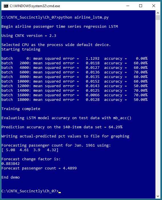
Figure 7-1: Time Series Regression Using a Neural Network

The screenshot in Figure 7-1 shows an example of time series regression using an LSTM (long short-term memory) deep neural network. The data is a well-known dataset of the monthly number of international airline passengers, from January 1949 through December 1960. The data and resulting prediction model are graphed in Figure 7-2.

Unlike the other examples in this e-book, in time series regression there isn’t a clear distinction between feature/predictor values and class/values-to-be predicted. Each predicted value is based on one or more previous values.

The distinction is a bit subtle. In the graph in Figure 7-2, the first passenger count is 1.12 (112,000 passengers) for month 1, and the second passenger count is 1.18 for month 2. It’s not correct to think that f(1) = 1.12 and f(2) = 1.18, and so on for some function f(t). Each passenger count is part of the series of values, and not an explicit function of a time variable of some sort.

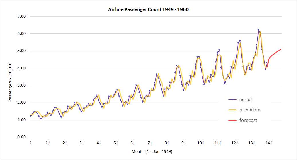
Figure 7-2: Time Series Regression Actual vs. Predicted

After a time series regression model has been created, it is typically used in one of two ways. The model can be used to identify anomalous data points in the historical data, or the model can be used to forecast one or more time steps ahead (sometimes called extrapolation). In the demo, there aren’t any clearly anomalous data points. The forecast for January 1961 is 4.49 (449,000) passengers.

Preparing the airline passenger data 

The airline passenger dataset appears to have first been published in the 1976 book Time Series Analysis: Forecasting and Control by Box and Jenkins; however, it’s not clear exactly where the authors obtained the raw data. The 144-item dataset can be found in several formats in many places on the Internet.

One form of the raw data is:

"1949-01";112
"1949-02";118
"1949-03";132
. . .

The LSTM time series regression demo program uses a rolling window technique, which is best explained by example. The data file used by the demo looks like:

|prev 1.12 1.18 1.32 1.29 |next 1.21 |change 1.08035714
|prev 1.18 1.32 1.29 1.21 |next 1.35 |change 1.14406780
|prev 1.32 1.29 1.21 1.35 |next 1.48 |change 1.12121212

The prev, next, and change tags were inserted so that the data could be easily processed by a CNTK Reader object. Each sequence of four consecutive data points is used as the predictor set for the next data point. Here the size of the input sequence is set to 4. The sequence size for LSTM is a free parameter, and must be determined by trial and error.

Each raw passenger count has been normalized by dividing by 100,000, so 1.12 means 112,000 passengers. Almost everything about time series regression problems is tricky; standard min-max and z-score normalization are often ineffective. You can find the complete dataset used by the demo program in the Appendix to this e-book.

The LSTM does not predict the next passenger count directly. Instead, the model predicts a change factor relative to the first item in the input sequence. For example, the first set of four input values are (1.12, 1.18, 1.32, 1.29) and the predicted change value is 1.08035714, which means that the next predicted passenger count is 1.12 * 1.08035714 = 1.2100, as shown in the data. The data item identified by the next tag is 1.21, and is the raw actual next count. The actual passenger count values are included only for convenience when computing an accuracy metric—the model predicts a change factor, not a count.

After formatting the 144 raw data points, there are 140 data sequences (the first four items have no predictors). Notice that setting up rolling window data results in some duplication of data because most data points appear four times. An alternative approach is to just maintain a single sequence (on file or in memory) and programmatically read from that sequence. But in most time series regression problem scenarios, there isn’t a huge amount of data, so the convenience of using duplicate data often outweighs the minor inefficiency.

LSTM networks

Unlike regular neural networks, LSTM networks maintain state. Informally, LSTM networks accept a sequence as input and remember a bit of their previous input and output values. LSTM networks are one of several types of recurrent neural networks.

LSTM networks were designed to work with natural language data. For example, suppose you were asked to predict the next word in the sentence, “I’m taking lessons in _____.” Without any context, you’d have a difficult time making an accurate prediction. But suppose knew a previous sentence in the paragraph was, “I’m looking forward to my trip to Spain.” You’d probably predict the unknown word in the other sentence is “Spanish.”

Let me emphasize that the use of LSTM networks for time series regression is speculative, and at the time this e-book is being written, there are no definitive research results that indicate whether LSTM networks work better than, or worse than, traditional techniques. However, using LSTMs for time series regression appears promising. Additionally, using an LSTM network with numeric data is easier than working with natural language data, and gives you a good introduction to LSTMs.

The CNTK library supports LSTM networks. An LSTM cell is shown in Figure 7-3. Even a quick glance at the figure should convince you that LSTMs are complicated, and that implementing an LSTM network from scratch would be extremely challenging. In the figure, the X_t vector represents an input sequence of four consecutive airline passenger counts. The Y_t vector represents four output values. To compute output values, the LSTM cell uses the input sequence, plus the previous output values (the “short-term” memory), plus a state that holds information about all previous input and output values (the “long” memory).

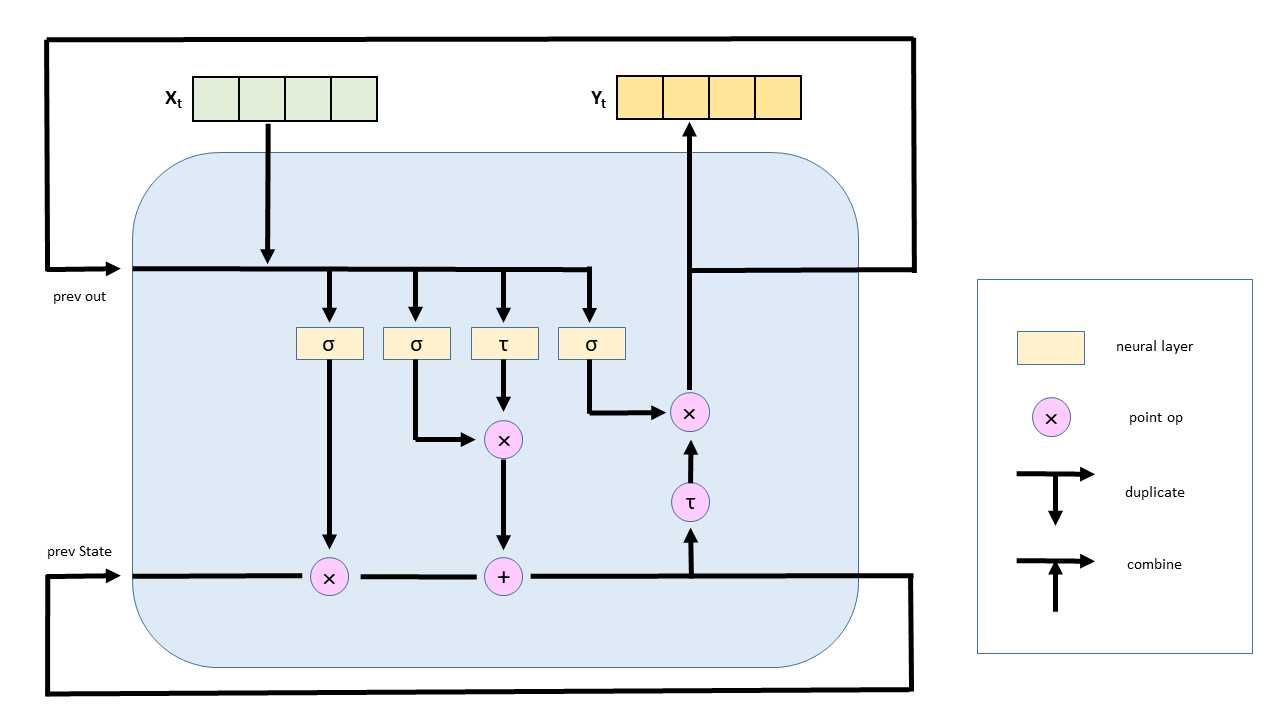
Figure 7-3: An LSTM Network Cell  

The internal structure of an LSTM cell uses sigmoid neural layers, called gates, to control how much information is remembered and how much information is forgotten. A tanh neural layer holds state information. An LSTM cell also uses vector multiplication and addition.

The LSTM time series regression program

The LSTM time series regression program code is presented in Code Listing 7-1. After importing the required NumPy and CNTK packages, the demo program defines a helper function to read data from a CNTK format file into a mini-batch object:

def create_reader(path, input_dim, output_dim, rnd_order, sweeps):
  x_strm = C.io.StreamDef(field='prev', shape=input_dim, is_sparse=False)
  y_strm = C.io.StreamDef(field='change', shape=output_dim, is_sparse=False)
  z_strm = C.io.StreamDef(field='next', shape=output_dim, is_sparse=False)
  streams = C.io.StreamDefs(x_src=x_strm, y_src=y_strm, z_src=z_strm)
  deserial = C.io.CTFDeserializer(path, streams)
  mb_source = C.io.MinibatchSource(deserial, randomize=rnd_order, max_sweeps=sweeps)
  return mb_source

Notice that create_reader() defines three streams instead of the usual two streams. It’s not necessary to define a stream that corresponds to each tag in a CNTK-format data file. If you don’t intend to use a field in a CNTK-format data file, you can ignore the field by not creating a stream for the field.

Code Listing 7-1: Time Series Regression

Because the output of the demo LSTM network is a numeric value, it’s necessary to implement a custom accuracy function if you want to measure accuracy. The demo program defines a function mb_accuracy() (“mini-batch accuracy”) that computes the percentage of correct output values, given a mini-batch of input and output values, and a model to compute predicted output values:

def mb_accuracy(mb, x_var, y_var, model, delta):
  num_correct = 0; num_wrong = 0
  x_mat = mb[x_var].asarray()  # batch_size x 1 x features_dim
  y_mat = mb[y_var].asarray()  # batch_size x 1 x 1
  for i in range(len(mb[x_var])):
    v = model.eval(x_mat[i])           # 1 x 1 predicted change factor
    y = y_mat[i]                       # 1 x 1 actual change factor
    if np.abs(v[0,0] - y[0,0]) <  delta:  # close enough?
      num_correct += 1
    else:
      num_wrong += 1
  return (num_correct * 100.0) / (num_correct + num_wrong)

Recall that the LSTM network predicts a change factor, not a passenger count. So the accuracy function computes accuracy based on the predicted change factor, not the predicted passenger count. The actual next-month passenger count values in the data file are not used at all.

In the main() function, the demo program prepares to create an LSTM model with these statements:

  train_file = ".\\Data\\airline_train_cntk.txt"
 
  input_dim = 4   # context pattern window
  output_dim = 1  # passenger count increase/decrease factor
  X = C.ops.sequence.input_variable(input_dim)  # sequence of 4 items
  Y = C.ops.input_variable(output_dim)  # pct change from X[0]
  Z = C.ops.input_variable(output_dim)  # actual next passenger count

The number of values in each input sequence is set to 4. LSTMs can handle variable-sized input sequences. Such sequences often occur when processing natural language (sentence length for example). But for numeric data, a fixed sequence/window size is much more common.

When using an LSTM, instead of creating an input Variable object using the cntk.ops.input_variable() function, you create a special Variable object using the cntk.ops.sequence.input_variable() function.

The LSTM network cell is created like so:

  model = None
  with C.layers.default_options():
    model = C.layers.Recurrence(C.layers.LSTM(shape=256))(X)
    model = C.sequence.last(model)
    model = C.layers.Dense(output_dim)(model)  

An LSTM cell is created inside a Recurrence layer so that its output values and state are fed back as inputs as shown in Figure 7-3. The shape=256 argument to LSTM() is the size of the state-output and internal tanh layer that remembers previous inputs and output values. Instead of just passing an integer directly, that argument is sometimes passed indirectly as a variable, named something like hidden_dim.

Roughly speaking, larger values of the shape parameter mean the LSTM remembers more, but this isn’t necessarily always a good thing. For time series regression, the network probably won’t benefit from remembering input patterns far in the past.

Using the sequence.last() function is syntactically required. The last() function returns the last state-output in the LSTM cell (256 values), because only the last state generated by the set of input sequences is wanted.

LSTM networks often use a dropout layer that randomly drops nodes during training in order to reduce the likelihood of model overfitting. The demo doesn’t use dropout.

The last layer in the network is a standard Dense layer that adds a final node and condenses the 256 final-state values to a single value. Technically this isn’t entirely necessary, but adding an extra layer adds additional weights and an additional bias value, which in theory, gives the model more predictive power.

You could add multiple Dense layers, for example:

  model = C.layers.Recurrence(C.layers.LSTM(shape=256))(X)
  model = C.sequence.last(model)
  model = C.layers.Dense(10)(model)
  model = C.layers.Dense(output_dim)(model)

And you could add additional Recurrence layers, for example:

  model = C.layers.Recurrence(C.layers.LSTM(shape=256))(X)
  model = C.layers.Recurrence(C.layers.LSTM(shape=256))(model)
  model = C.sequence.last(model)
  model = C.layers.Dense(output_dim)(model) 

Little is known about exotic LSTM network architectures, and investigating these architectures is an active area of deep neural network research.

Training an LSTM network

After the LSTM network is created, Learner and Trainer objects are created in the usual way:

  learn_rate = 0.01
  tr_loss = C.squared_error(model, Y)
  learner = C.adam(model.parameters, learn_rate, 0.99)
  trainer = C.Trainer(model, (tr_loss), [learner])

As a rule of thumb, as network architectures increase in size and complexity, the more important advanced Learner algorithms become. The demo uses the Adam (adaptive moment estimation) learner, which is a good first try when working with LSTM networks. The 0.99 argument is assigned to the adam() function’s momentum parameter, but somewhat confusingly is described by the CNTK documentation as the beta1 parameter. Choosing reasonable values for advanced learning functions when there are no default values requires research, trial and error, and patience.

The demo program creates a reader for the time series training data like so:

  rdr = create_reader(train_file, input_dim, output_dim,
    rnd_order=True, sweeps=C.io.INFINITELY_REPEAT)

  airline_input_map = {
    X : rdr.streams.x_src,
    Y : rdr.streams.y_src
  }

The create_reader() function is called using rnd_order=True, which means that each batch of training items will be processed in a random order. This seems counterintuitive because the training data is one big sequence of values. In discussions with my colleagues, there is roughly a 50-50 split in opinion regarding whether training data should be processed in a random order or in a sequential order. As was the case with simple neural networks when they were new (in the 1980s), many fundamental concepts about LSTM networks are not currently well understood.

The actual training of the LSTM network for time series regression is performed by these statements:

  max_iter = 20000
  batch_size = 10
  print("Starting training \n")
  for i in range(0, max_iter):
    curr_mb = rdr.next_minibatch(batch_size, input_map=airline_input_map)
    trainer.train_minibatch(curr_mb)
    if i % int(max_iter/10) == 0:
      mcee = trainer.previous_minibatch_loss_average
      acc = mb_accuracy(curr_mb, X, Y, model, delta=0.10)  # program-defined
      print("batch %6d: mean squared error = %8.4f  accuracy = %7.2f%%" \
        % (i, mcee, acc))
  print("\nTraining complete")

  mdl_name = ".\\Models\\airline_lstm.model"
  model.save(mdl_name)  # CNTK v2 format is default

Typically, training an LSTM network requires many more training iterations than training a single hidden layer neural network. Monitoring error/loss during training is critically important because when working with LSTM networks, based on my experience, training failure is the rule rather than the exception. The demo prints error 10 times during training: int(max_iter/10).

The demo program saves the trained model after training completes (using the default CNTK v2 format). An alternative is to also save intermediate models during training, every so often. For example, inside the if condition in the code above, you could write:

  mdl_name = ".\\Models\\airline_lstm_" + str(i) + ".model"
  model.save(mdl_name)

And instead of embedding just the training iteration into the intermediate model name, you could also embed information such as the loss/error associated with the model. The point is that for non-demo datasets, training can take hours or days, and saving intermediate models is necessary in practice. CNTK supports a checkpoint mechanism that is outside the scope of this e-book.

The average model accuracy on the current batch of 10 training items is printed every so often. After training, the demo program also computes and prints the model accuracy on the entire 140-item dataset, using the program-defined mb_accuracy() function. In a non-demo scenario, you’d likely also want to compute and print the average loss/error for the entire dataset. For example, you could code a program-defined function:

def mb_error(mb, x_var, y_var, model):
  sum_sq_err = 0.0
  x_mat = mb[x_var].asarray()  # batch_size x 1 x features_dim
  y_mat = mb[y_var].asarray()  # batch_size x 1 x 1
  for i in range(len(mb[x_var])):
    v = model.eval(x_mat[i])           # 1 x 1 predicted change factor
    y = y_mat[i]                       # 1 x 1 actual change factor
    sum_sq_err += (v[0,0] - y[0,0]) * (v[0,0] - y[0,0])
  return sum_sq_err / len(mb[x_var])

It would likely be a mistake to try and use the built-in previous_minibatch_loss_average property of the Trainer object, because you’d have to call the train() method, which would modify the trained model.

Prediction and forecasting

When performing time series regression, it’s almost always useful to graph results. After training, the demo LSTM program walks through the 140-item training data, computes a predicted passenger count, and then writes actual count and predicted count pairs to a text file.

First, the program prepares the analysis:

  print("\nWriting actual-predicted passenger counts to file for graphing")
  fout = open(".\\Data\\actual_predicted_lstm.txt", "w")
  rdr = create_reader(train_file, input_dim, output_dim,
    rnd_order=False, sweeps=1)
  airline_input_map = {
    X : rdr.streams.x_src,
    Y : rdr.streams.y_src,
    Z : rdr.streams.z_src   # actual next passenger count
  }
  num_items = 140
  all_items = rdr.next_minibatch(num_items, input_map=airline_input_map)

Even though the LSTM network model predicts a change factor rather than a direct passenger count, it makes more sense to graph actual-predicted passenger counts rather than actual-predicted change values (although you could graph both).

Instead of computing an actual passenger count from the actual change factor and the first value of the input sequence, the demo program reads the actual counts, which were stored in the training data file for convenience. Notice the input map for the Reader object sets up all three data streams. Next, the demo program extracts the input sequences, the actual changes, and the actual next count data into three matrices:

  x_mat = all_items[X].asarray()
  y_mat = all_items[Y].asarray()
  z_mat = all_items[Z].asarray()

Recall that all_items is a CNTK mini-batch object which is implemented as a dictionary object, and the X, Y, and Z Variable objects are used as keys. Next, each item is processed:

  for i in range(all_items[X].shape[0]):  # each item in the batch
    v = model.eval(x_mat[i])           # 1 x 1 predicted change
    y = y_mat[i]                       # 1 x 1 actual change
    z = z_mat[i]                       # actual next count
    x = x_mat[i]                       # first item in sequence
    p = x[0,0] * v[0,0]                # predicted next count
    fout.write("%0.2f, %0.2f\n" % (z[0,0], p))

  fout.close()

The eval() function computes the predicted change values into v, so the predicted passenger count is the first item in the current sequence, x[0,0], times v[0,0], because both values are returned into 1´1 matrices. In practice, you will spend a lot of time determining the shape of different CNTK objects using the shape property and a print() function.

Each actual-predicted comma-separated pair is written to the specified text file. An alternative is to store actual-predicted pairs into a Python list using the append() or insert() function.

After writing actual-predicted data to the text file, I opened the file with Excel and created the graph shown in Figure 7-2. An alternative is to programmatically create a graph from within your script using the Python matplotlib package. Many of the CNTK documentation examples use this approach. However, matplotlib code can obscure the main ideas of CNTK model creation, training, and evaluation, so I’ve used an external technique to create the graph.

In time series regression, making a prediction for input values beyond the range of the input values in the training data is usually called forecasting or extrapolation. The demo program predicts the change for the first time period past the training data (January 1961, month 141) and then uses the change to compute the predicted next passenger count:

  in_seq = np.array([[5.08, 4.61, 3.90, 4.32]], dtype=np.float32)  # last 4 actual
  print("\nForecasting passenger count for Jan. 1961 using: ")
  print(in_seq[0])
  pred_change = model.eval({X: in_seq})
  print("\nForecast change factor is: ")
  print("%0.6f " % pred_change[0,0])
  pred_count = in_seq[0,0] * pred_change[0,0]
  print("Forecast passenger count = %0.4f" % pred_count)  

The in_seq 1´4 array holds the last four normalized actual passenger counts. The array is passed to the eval() function via the X key to create an anonymous dictionary object. The array could have been passed directly. The return value is a 1´1 matrix that holds the predicted change. That change value is multiplied by the first item in the input sequence to determine the predicted passenger count.

In many situations, you only want to predict one time-unit ahead. However, you can extrapolate as many time units as you wish. The short program in Code Listing 7-2 extrapolates eight time units past the training data.

Code Listing 7-2: Extrapolating Time Series

As you can see in the graph in Figure 7-2, you must use great caution when extrapolating time series data, because the accuracy of the predictions will often degrade quickly.

Exercise

The Appendix of this e-book has raw data for monthly initial unemployment claims for King County Washington (Seattle area) from January 2005 through December 2014. Using the program in Code Listing 7-1 as a guide, create an LSTM time series regression model.

The raw data came from here.

The raw comma-delimited data has 120 items and looks like:

8/1/2007,6110
9/1/2007,5298
. . .
11/1/2014,6993
12/1/2014,7978

You will have to decide how to normalize the data, and how to set up a CNTK-format data file. I suggest using Excel or a similar spreadsheet to preprocess the raw data.