Logistic Regression

Logistic regression is one of the simplest machine-learning techniques. Logistic regression is a technique for a binary classification problem: to create a prediction model in situations where the value of the variable to predict (often called the label in machine learning terminology) can be one of just two categorical values. For example, you might want to predict the sex of a person (male or female) based on the person’s age, years of education, and annual income.

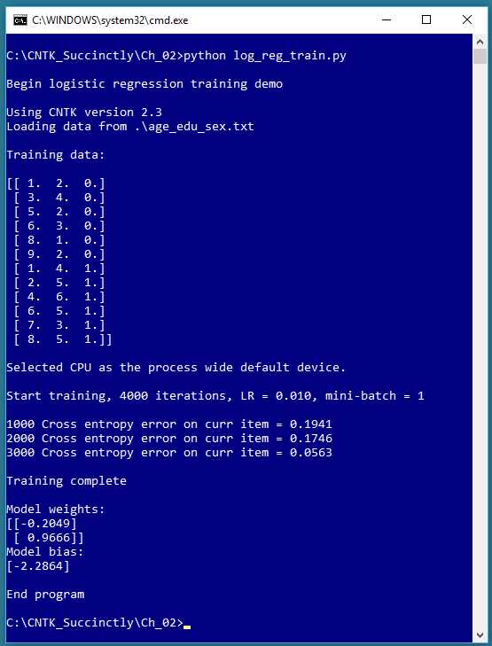
Figure 2-1: Logistic Regression Using CNTK

The screenshot in Figure 2-1 shows a simplified example of logistic regression. The demo program begins by loading 12 data items into memory. Each item represents a person’s age, education, and sex. For example, the first data item is (1.0, 2.0, 0), which is a person with age = 1.0, education = 2.0, and sex = female.

Age and education are the predictor variables (often called features in CNTK and machine learning terminology). The values of the feature variables have been normalized in some way so that their magnitudes are all between 1.0 and 9.0. The variable-to-predict (often called the class or class label) is encoded with female = 0 and male = 1.

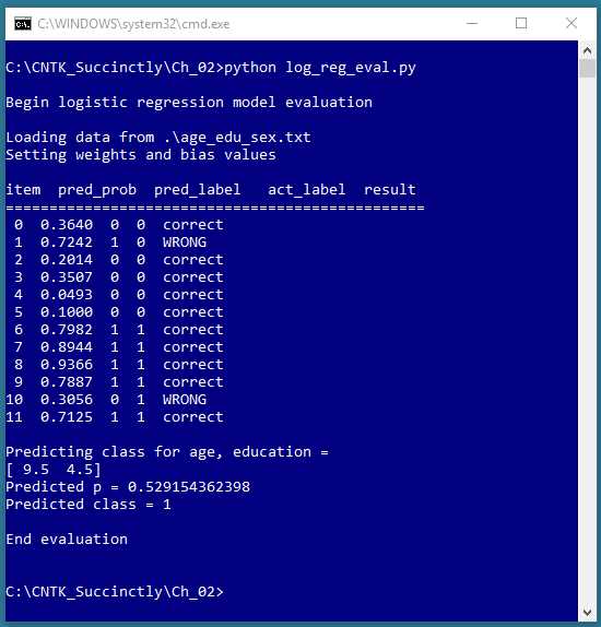
Figure 2-2: Evaluating the Logistic Regression Model

The CNTK demo training program creates a logistic regression prediction model using 4,000 iterations of the stochastic gradient descent algorithm with binary cross-entropy error. After training completed, the demo displayed the values of the weights (-0.2049, 0.9666) and the value of the bias (-2.2864) that define the logistic regression model.

The screenshot in Figure 2-2 shows an evaluation of the trained logistic regression model. The program walks through each of the 12 training items, and computes and displays a prediction probability, the associated predicted class, the actual class, and a tag indicating if the prediction is correct or incorrect. The logistic regression prediction model correctly predicted 10 of the training items, for a classification accuracy of 10 / 12 = 83%.

After evaluating the model, the program shown in Figure 2-2 makes a prediction for a new, previously unseen person. The unknown item has normalized age = 9.5 and normalized education = 4.5. The prediction probability is 0.5291 and so the predicted class is 1 (male).

Understanding logistic regression

In order to understand the CNTK code that generated the output shown in Figures 2-1 and 2-2, you need a basic understanding of logistic regression. The key ideas are best explained by example. Suppose you want to predict the credit worthiness of a loan application (0 = reject, 1 = approve) based on the application’s x1 = debt, x2 = income, x3 = credit rating. In logistic regression, you determine a weight value, w, for each feature, and a single bias value b.

Suppose x1 = 3.0, x2 = -2.0, and x3 = 1.0. And suppose you determine that w1 = 0.65, w2 = 1.75, w3 = 2.05, and b = 0.33. To compute the predicted class, you first compute z = (x1 * w1) + (x2 * w2) + (x3 * w3) + b:

z = (3.0)(0.65) + (-2.0)(1.75) + (1.0)(2.05) + 0.33
   = 1.95 - 3.50 + 2.05 + 0.33
   = 0.83

Next you compute p = 1.0 / (1.0 + exp(-z)) where the exp() function is Euler’s number, e (~2.71828) raised to a power:

p = 1.0 / (1.0 + exp(-0.83))
   = 1.0 / (1.0 + 0.4360)
   = 1.0 / 1.43630
   = 0.6963

The p-value can be interpreted as the probability that the class is 1. Put another way, if p < 0.5 the prediction is class = 0, otherwise (if p >= 0.5) the prediction is class = 1.

OK, but where do the weights and bias values come from? To determine the values of the weights and bias, you must obtain a set of training data that has known input predictor values, and known, correct class label values. Then you use an algorithm (typically gradient descent, or a variation called stochastic gradient descent) to find values for the weights and bias so that computed output values closely match the known correct class labels.

An important aspect of logistic regression training is measuring the error between computed output values (using a set of weights and a bias) and the correct class label. Suppose, for a given set of input values and a given set of weights and bias values, the computed p value is 0.7000 and the known correct class label is 1. You could compute a squared error:

se = (1 - 0.7000) * (1 - 0.7000)
     = 0.09

And in fact, this approach can be used with logistic regression. However, for rather complex technical reasons, it’s considered preferable to use what’s called binary cross-entropy error (also called log-loss).

For the numeric example above (p = 0.7000, c = 1), binary cross-entropy error is calculated as:

cee = - [c * ln(p)] + [(1-c) * ln(1-p)]
       = - [1 * ln(0.7000)] + [0 * ln(0.3000)]
       = -ln(0.7000)
       = 0.3567

Cross-entropy error is a bit difficult to interpret, but smaller values mean smaller error (which means a more accurate prediction). As you’ll see shortly, CNTK has functions that support both squared error and cross-entropy error. The key thing to remember is that when performing logistic regression training is that unless you have an existing system committed to using squared error, it’s recommended that you use binary cross-entropy error, and smaller values are better.

Setting up the training data

The training data used by the programs shown in Figures 2-1 and 2-2 is graphed in Figure 2-3 and is:

1.0, 2.0, 0
3.0, 4.0, 0
5.0, 2.0, 0
6.0, 3.0, 0
8.0, 1.0, 0
9.0, 2.0, 0
1.0, 4.0, 1
2.0, 5.0, 1
4.0, 6.0, 1
6.0, 5.0, 1
7.0, 3.0, 1
8.0, 5.0, 1

When using CNTK for logistic regression, it’s up to you to prepare your training data, including normalizing feature values, and encoding class labels as 0 or 1. For example, the raw data might have resembled:

25.0, 12, female
37.0, 16, male
. . .

The demo program uses only two predictor variables, just to keep things simple, and so that the data can be displayed in a two-dimensional graph. Logistic regression can be used with any number of predictor variables. The predictor variables must be numeric, but it is possible to convert non-numeric predictor values into numeric values so that you can use logistic regression.

Compared to other binary classification techniques, the main advantage of logistic regression is simplicity. The primary disadvantage of logistic regression is that it only works well with data that is linearly separable. Conceptually, logistic regression finds a straight line that separates the two classes. For the demo data, no straight line will do better than 10 of 12 correct predictions.

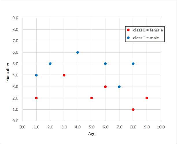
Figure 2-3: Data for Logistic Regression

Feature normalization and class encoding are explained in detail in Chapter 3. The data was copied into Notepad and saved as age_edu_sex.txt on a local machine. In a non-demo scenario, you might have hundreds, or thousands of training items.

Creating a logistic regression model

The program code that generated the screenshot shown in Figure 2-1 is presented in Code Listing 2-1. The program begins by commenting the name of the file and version of CNTK used, and importing the NumPy and CNTK packages:

# log_reg_train.py
# logistic regression age-education-sex synthetic data
# CNTK 2.3
import numpy as np
import cntk as C

In a non-demo scenario, you’d want to include additional details. The program structure consists of a single main function, with no helper functions:

def main():
  print("\nBegin logistic regression training demo \n")
  ver = C.__version
  print("Using CNTK version " + str(ver))
  . . .
  print("End program ")
if __name__ == "__main__":
  main()

I indent with two spaces rather than the normal four spaces because of page-width limitations. All normal error checking has been removed to keep the main ideas clear. Because CNTK is young and under active development, it’s good practice to indicate which version is being used in a code comment, and to programmatically verify the version, as shown.

Code Listing 2-1: Logistic Regression Training

Next, the program loads the training data into memory:

  # training data format:
  # 4.0, 3.0, 0
  # 9.0, 5.0, 1
  # . . .

  data_file = ".\\age_edu_sex.txt"
  print("Loading data from " + data_file + "\n")
  features_mat = np.loadtxt(data_file, dtype=np.float32, delimiter=",",
    skiprows=0, usecols=[0,1])
  labels_mat = np.loadtxt(data_file, dtype=np.float32, delimiter=",",
    skiprows=0, usecols=[2], ndmin=2)

The training data is located in the same directory as the training program. The CNTK training functions expect training data to be supplied in two matrices: one for the features, and one for the class labels. The demo uses the numpy.loadtxt() function. Note that this technique only works if your training data is small enough to be completely stored in memory. For large datasets, CNTK supports a Reader object, which is described in Chapter 4.

Most machine learning models use the float32 data type, rather than the more common float64 type, because the extra precision gained by using 64 bits is rarely worth the performance penalty incurred. The skiprows parameter is useful when a dataset has one or more header lines. Notice that columns are zero-base indexed.

The shape of the features_mat matrix is determined by the structure of the data file, and so in this case is 12´2 (12 rows, 2 columns). Notice the ndmin=2 (“minimum dimensions”) for the labels_mat matrix. Without that parameter, loadtxt() would infer a one-dimensional vector return type rather than the required 12´1 two-dimensional matrix.

Incompatible and incorrect matrix shapes are a very common source of CNTK errors. One way to track down matrix shape errors during development is to print shape information using the shape property, for example, print(labels_mat.shape), which will display (12, 1).

After loading the training data into memory, the program displays the data like so:

  print("Training data: \n")
  combined_mat = np.concatenate((features_mat, labels_mat), axis=1)
  print(combined_mat); print("")

The concatenate() function combines two or more arrays or matrices. This is done, instead of displaying the features matrix and the labels matrix separately, only to make the display easier to read. Instead of printing the entire combined matrix, you could display just the first three rows using special Python syntax: print(combined_mat[(0,1,2),:]) or print(combined_mat(range(0,3),:]). You can interpret either as, “Rows 0, 1, and 2, and all columns.”

Next, the training program creates an (untrained) logistic regression model that is compatible with the training data:

   # create model
  features_dim = 2  # x0, x1
  labels_dim = 1    # always 1 for log regression
  X = C.ops.input_variable(features_dim, np.float32)    # cntk.Variable
  y = C.input_variable(labels_dim, np.float32)    # correct class value
  W = C.parameter(shape=(features_dim, 1))   # trainable cntk.Parameter
  b = C.parameter(shape=(labels_dim))
  z = C.times(X, W) + b        # or z = C.plus(C.times(X, W), b)
  p = 1.0 / (1.0 + C.exp(-z))  # or p = C.ops.sigmoid(z)
  model = p  # create an alias

The features_dim variable holds the number of predictor variables (two, for age and education in this case). The labels_dim holds the number of class labels. For logistic regression, this will always be 1 (even though the class label can take one of two possible values, 0 or 1, corresponding to female and male­­—one variable, two values). Neither dim variable name is a CNTK keyword so you can use names like x_dim and y_dim if you wish.

The CNTK input_variable() function creates storage to hold feature and label values. Notice that the assignment to object X uses the fully qualified name C.ops.input_variable() but the assignment to object y uses the shortcut syntax C.input_variable(). An alternative approach is to import specific functions and omit the qualification. For example:

import numpy as np
from cntk.ops import input_variable
. . .
X = input_variable(features_dim, np.float32)

The input_variable() function, like most CNTK functions, has a large number of parameters that can be omitted in a function call, because most parameters have default values, which makes the an explicit inclusion of those parameters optional. For example, input_variable() has optional parameters needs_gradient, is_sparse, dynamix_axes, and name. In fact, the dtype (data type) parameter has default value np.float32, so that argument could have been omitted, too.

The W matrix holds the logistic regression weights, and the b scalar holds the single bias value. Note that both are created with a call to the parameter() function, which means that when a CNTK training method is called, those object values will be updated automatically.

The logistic regression model is specified by computing a z value as the sum of products of weight and feature values, plus the bias b. The probability value, p, is computed as described previously. Note that I use the CNTK exp() function rather than the NumPy np.exp() function or the base Python math.exp() function; I could have used any of these three.

The function f(x) = 1.0 / (1.0 + exp(-x)) occurs often in machine learning, and is called the logistic sigmoid function (sometimes not entirely correctly abbreviated to just sigmoid). CNTK has a built-in sigmoid() function, so the code that computes p can be written as:

p = C.ops.sigmoid(z)

At this point, at a low level, p represents the probability that the class has value 1, and at a higher level of abstraction, p represents the overall logistic regression model. The demo program creates a name-friendly alias by assigning object p to object model. This is completely optional and is done just for readability. CNTK also has an ops.alias() function you can use.

Training a logistic regression model

After reading the training data into memory and creating a logistic regression model, the next step is to train the model. The demo program continues by creating a Learner and a Trainer object:

  # create Learner and Trainer
  ce_error = C.binary_cross_entropy(model, y)
  fixed_lr = 0.010
  learner = C.sgd(model.parameters, fixed_lr)
  trainer = C.Trainer(model, (ce_error), [learner])
  max_iterations = 4000

You can think of a Learner as an algorithm to minimize error, and a Trainer as an object that uses the Learner to compute the weights and bias values. The demo program uses the binary cross-entropy function from the CNTK losses package to measure the error between computed output probabilities and known correct label values (0 or 1). If you wanted to use squared error, the code could be s_error = C.squared_error(model, y).

The demo sets up a stochastic gradient descent learning algorithm using the sgd() function. CNTK supports many advanced learning algorithms such as adadelta(), adam(), and nesterov(). Advanced algorithms are most often used with deep neural networks. Stochastic gradient descent is the simplest learning algorithm, and generally works well for logistic regression problems.

The sgd() function requires a learning rate, which is a value that influences how much the weights and bias value change on each training iteration. The value of the learning rate must be determined by trial and error. If the learning rate is too small, training will be very slow. If the learning rate is too large, training may skip over a good result.

Instead of using a fixed learning rate, you can specify a learning rate schedule where the learning rate varies. Typically, this is a relatively large learning rate during the early iterations, and then smaller rate(s) during later iterations.

After a Learner object has been created, it is passed as an argument to the trainer() function to create a Trainer object. The second parameter to trainer() is a tuple, as indicated by the parentheses, because you can pass more than one error function. For linear regression, you should pass the binary cross-entropy function (or squared error). You can optionally create a second error function that measures classification error—the percentage of incorrect predictions made. For example:

clas_err = C.classification_error(model, y)
trainer = C.Trainer(model, (ce_error, clas_err), [learner])

However, as you’ll see shortly, because the demo program adjusts weights and bias values after processing a single training item, computing classification accuracy is better done in a different way.

The third parameter to trainer() is a list, as indicated by the square brackets, because you can pass multiple Learner objects. This technique is usually used with deep neural networks— different parts of the network can use different learner algorithm objects.

Stochastic gradient descent is an iterative technique, so you must have some stopping condition. The simplest approach is to specify a fixed number of training iterations. The number of iterations must be determined by trial and error.

After the learner and trainer objects are created, the demo program trains the logistic regression model like so:

   # train
  print("\nStart training, 4000 iterations, LR = 0.010, mini-batch = 1 \n")
  np.random.seed(4)
  N = len(features_mat)

  for i in range(0, max_iterations):
    row = np.random.choice(N,1)  # pick a random row from training items
    trainer.train_minibatch({ X: features_mat[row], y: labels_mat[row] })  

    if i % 1000 == 0 and i > 0:
      mcee = trainer.previous_minibatch_loss_average
      print(str(i) + " Cross-entropy error on curr item = %0.4f " % mcee)

  print("\nTraining complete \n")

When training a model, you must decide how many training items to use for each weight and bias update operation. For logistic regression, the most common approach (and the one used by the demo) is to update weights and bias values after processing a single training item. This is often called online training. An alternative is to process all training items and then perform an update operation. This is often called batch training.

A third approach is to process a certain number of training items—for example, four or five—before updating. This is often called mini-batch training. Notice that mini-batch training with a batch size equal to 1 is equivalent to online training, and that mini-batch training with a batch size equal to the size of the training dataset is equivalent to batch training.

When using the online or mini-batch approach, it’s important that the training items be visited in random order. The demo sets np.random.seed to 4 so that results are reproducible. The seed value of 4 was used only because it gave a representative demo output. Inside the training loop, function np.random.choice() is used to select a single row index.

The train_minibatch() function accepts the predictor values, creates an anonymous dictionary object with X as the key, and the known correct class label (an anonymous dictionary object with y as the key). Behind the scenes, train_minibatch() computes a predicted output, then uses binary cross entropy to update each weight and bias value slightly, governed by the learning rate.

When training a model, it’s important to display the current error so you can catch situations where training isn’t working. Training failure is very common. The demo uses the previous_minibatch_loss_average property to display the binary cross-entropy error for the previous training item, once every 1,000 iterations. The previous item is used rather than the current item because of the internal architecture of CNTK. In a non-demo scenario, you’d likely display error more frequently, for example, once every 100 iterations.

Note that when using online training, because you’re only processing one training item at a time, the error value will be quite volatile. What you hope to see are error values that generally decrease. What you don’t want to see are error values that don’t really change, or worse, values that steadily increase.

When using online training, it’s not too helpful to display the classification error, or its complement, classification accuracy, because the accuracy applies to a single training item and will be either 0% (if the item is incorrectly predicted) or 100% (for a correct prediction).

The online training algorithm used in the demo selects a random row from the training data, 4,000 times. This doesn’t guarantee that each training item will be used the same number of times. A more sophisticated approach is to walk through each training item, in random order, and then repeat that process several times. For example:

  # train
np.random.seed(0)
N = len(features_mat)
for sweep in range(0, 100):
   indices = np.random.choice(N, N, replace=False)
   for idx in indices:
     trainer.train_minibatch({ X: features_mat[idx], y: labels_mat[idx] })
   mcee = trainer.previous_minibatch_loss_average
   print(" Cross-entropy error on curr item = %0.4f \n" % mcee)

Because there are N = 12 training items, the np.random.choice() function generates an array of indices, from 0 to 11, in random order. The training item at each index is processed, and then another set of indices in random order is generated. This means there would be 100 * 12 = 1200 total update operations and each training item is used the same number of times.

The demo training program concludes by displaying the values of the two weights and the value of the bias:

  np.set_printoptions(precision=4, suppress=True)
print("Model weights: ")
print(W.value)
print("Model bias:")
print(b.value)
print("")

Notice that you can’t simply print W and b directly because they are CNTK objects of type Parameter, so you must use their value property. The values of W and b effectively define the logistic regression model so instead of just displaying them; you might want to write them to a text file so they can be retrieved by another program.

Using a trained logistic regression model

After a logistic regression model has been trained, you’ll usually want to evaluate it for classification accuracy, and eventually use it to make a prediction for new, previously unseen data. The program log_reg_eval.py that generated the output shown in Figure 2-2 is presented in Code Listing 2-2. Note that the \ character is used by Python for line continuation.

Code Listing 2-2: Evaluating a Trained Model

The evaluation program imports the numpy package but does not need the cntk package, because the classification accuracy of the trained model will be computed from scratch rather than by using the previous_minibatch_evaluation_average property of the CNTK Trainer object.

The evaluation program loads the training data into a features matrix and a class label matrix in exactly the same way as the training program. In many scenarios you will want to combine training and evaluation into the same program; two different programs are used here to emphasize the distinction between the two operations.

Next, the evaluation program sets the values of the weights and the bias that were determined by the training program:

  print("Setting weights and bias values \n")
weights = np.array([0.0925, 1.1722], dtype=np.float32)
bias = np.array([-4.5400], dtype=np.float32)
N = len(features_mat)
features_dim = 2

Notice that the evaluation program uses ordinary NumPy arrays rather than CNTK Parameter objects. Next, the evaluation program walks through each training item and computes the logistic regression probability:

  print("item  pred_prob  pred_label   act_label  result")
  print("================================================")
  for i in range(0, N):  # each item
    x = features_mat[i]
    z = 0.0
    for j in range(0, features_dim):  # each feature
      z += x[j] * weights[j]
    z += bias[0]
    pred_prob = 1.0 / (1.0 + np.exp(-z))
. . .

An alternative approach is to write a program-defined function to perform this calculation. For example:

def compute_p(x, w, b):
  z = 0.0
  for i in range(len(x)):
    z += x[i] * w[i]
  z += b
  p = 1.0 / (1.0 + np.exp(-z))
  return p

After computing the prediction probability for the current training item, the program determines the associated predicted 0 or 1 label, and compares that with the actual class label:

  . . .
  pred_label = 0 if pred_prob < 0.5 else 1
  act_label = labels_mat[i]
  pred_str = ‘correct’ if np.absolute(pred_label - act_label) < 1.0e-5 \
    else ‘WRONG’
  print("%2d  %0.4f  %0.0f  %0.0f  %s" % \
    (i, pred_prob, pred_label, act_label, pred_str))

Comparing the computed class with the actual class is a bit tricky because the actual class is type float32, so the comparison checks to see if the two values are within 0.00001 of each other rather than check for exact equality. In practice you can usually compare directly, for example: pred_str = ‘correct’ if pred_label == act_label else ‘WRONG.

If you’re new to Python, the conditional if-statements may look a bit odd. You could in fact use standard C-family language syntax, for example:

if np.absolute(pred_label - act_label) < 1.0e-5:
  pred_str = 'correct'
else:
  pred_str = 'WRONG'

Because there are only 12 training items, the evaluation program just displays correct or WRONG. In a non-demo scenario, you’d likely want to use counter variables and then compute classification accuracy code along the lines of class_acc = num_corr * 1.0 / (num_corr + num_wrong).

In some situations, you may want to compute and display the final average binary cross-entropy error for all training data. If you are using batch training, you can use the Trainer object’s previous_minibatch_loss_average property, and then use the last value. A more flexible approach is to use the trained model and walk through each training item, and compute error yourself. For example, you could modify the code in the evaluation program to include:

  sum_bcee = 0.0  # sum of binary cross-entropy error terms
  for i in range(0, N):  # each item
    x = features_mat[i]
    z = 0.0
    for j in range(0, features_dim):  # each feature
      z += x[j] * weights[j]
    z += bias[0]                      # add the bias
    p = 1.0 / (1.0 + np.exp(-z))      # prediction prob
    y = labels_mat[i]                 # actual label/prob
    if y == 1:
      sum_bcee += -np.log(p)
    else:
      sum_bcee += -np.log(1-p)
  mean_bcee = sum_bcee / N
  print("mean binary cross-entropy error = " + str(mean_bcee))

The demo programs in this chapter use only one set of training data. In most situations, you’d have an additional test dataset that is held out from training. You’d then evaluate the classification accuracy, and possibly the cross-entropy error, on the test data. If the classification accuracy of the test data is significantly worse than the classification accuracy of the training data, your model may be overfitted.

The entire point of logistic regression classification is to make a prediction using new, previously unseen data. The evaluation demo concludes by demonstrating one way to make a prediction:

  x = np.array([9.5, 4.5], dtype=np.float32)
  print("\nPredicting class for age, education = ")
  print(x)
  z = 0.0
  for j in range(0, features_dim):
    z += x[j] * weights[j]
  z += bias[0]
  p = 1.0 / (1.0 + np.exp(-z))
  print("Predicted p = " + str(p))
  if p < 0.5: print("Predicted class = 0")
  else: print("Predicted class = 1")

Notice that because the logistic regression model was trained using normalized age and education values, you make predictions using normalized feature values, (9.5, 4.5) in this example.

The prediction code doesn’t use any CNTK functionality; therefore, you can use this approach in any system. For example, you could write equivalent code in some C# program. The trained weights and bias values define the model, so they can be used anywhere.

Exercise

There are several repositories for standard benchmark datasets for machine learning. One well-known dataset is the Wisconsin Cancer data. Using the programs in Code Listing 2-1 and 2-2 as guides, create and evaluate a logistic regression prediction model for the Wisconsin Cancer dataset.

The raw data is located at the University of California at Irvine repository.

There are several different versions of the dataset, and the documentation is quite confusing. Use the version of the dataset that has 699 items. Each item has an ID number, followed by nine normalized predictor values, followed by a value of 2 or 4, where 2 = benign and 4 = malignant.

The data resembles the following:

1000025,5,1,1,1,2,1,3,1,1,2
1002945,5,4,4,5,7,10,3,2,1,2
. . .
1017122,8,10,10,8,7,10,9,7,1,4
1018099,1,1,1,1,2,10,3,1,1,2
. . .
897471,4,8,8,5,4,5,10,4,1,4

The demo program in Code Listing 2-1 just displays the weights and bias values to the shell. So when you evaluate the model as in Code Listing 2-2, you need to copy those values into the program. As an alternative, you might want to write the weights and bias values to a text file using the Python open() and write() functions, and then load them using the read() function.

CNTK has save() and load() functions that make this process easier. The process for saving and loading a trained model using CNTK functions is explained in Chapter 4.