Fundamental Concepts

---

In order to effectively use the CNTK deep-learning code library functions, you must have a basic grasp of a handful of key machine learning concepts. This chapter explains neural network architecture and input-output, error and accuracy, data encoding and normalization, batch and online training, model overfitting, and train-test validation. The screenshot in Figure 3-1 gives you an idea of what this chapter covers.

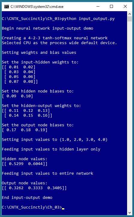
Figure 3-1: Neural Network Input-Output

Neural network architecture

The program that generate the output shown in Figure 3-1 is presented in Code Listing 3-1. A diagram that represents the demo program neural network is shown in Figure 3-2.

Code Listing 3-1: Neural Network Input-Output Mechanism

The demo program begins by importing the numpy and cntk packages. The set_printoptions() function suppresses printing very small values with scientific notation (such as 1.23e-6) and instructs print() to display floating point values to exactly two decimals.

Next, the demo prepares to create a neural network:

i_node_dim = 4
h_node_dim = 2
o_node_dim = 3

X = C.ops.input_variable(i_node_dim, np.float32)
Y = C.ops.input_variable(o_node_dim, np.float32)

The first three statements specify the number of input, hidden, and output nodes. The next two statements set up a CNTK type Variable object (X) to hold input data from a data source, usually a text file of training data, and a second Variable object (Y) to hold known, correct output values from the training data. The function name input_variable() may be a bit confusing—the “input” refers to input into the program from a data source, not necessarily input to a neural network.

Now the demo can create a neural network:

print("Creating a 4-2-3 tanh-softmax neural network")
h = C.layers.Dense(hnode_dim, activation=C.ops.tanh,
  name='hidLayer')(X)
o = C.layers.Dense(onode_dim, activation=C.ops.softmax,
  name='outLayer')(h)
nnet = o

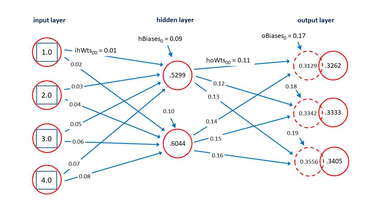
Figure 3-2: Neural Network Architecture

The Dense() function is used to create a fully connected layer of hidden nodes or output nodes, but not input nodes. The syntax is a bit strange. The X Variable object acts as input to the hidden layer h, and h acts as the input to the output layer o. The demo creates an alias of nnet to the output layer just for readability—the output of the neural network is conceptually the same as the network.

Notice that X is not really a layer of the network. If you wanted to create an explicit input layer, you could write:

i = X
h = C.layers.Dense(h_node_dim, activation=C.ops.tanh,
  name='hidLayer')(i)
o = C.layers.Dense(o_node_dim, activation=C.ops.softmax,
  name='outLayer')(h)
nnet = o  # or nnet = C.ops.alias(o)

The hidden layer is assigned a name property. This is optional, but useful in some situations. The hidden layer is configured to use tanh (hyperbolic tangent) activation. Activation functions are explained in the next section of this chapter. The output layer is also assigned a name, and is configured to use softmax activation. The nnet object is an alias for the output layer and can be omitted. You can also use the alias() function, as shown in the code comment.

Next, the demo program sets up the weights and biases. In the diagram in Figure 3-2, each blue arrow connecting a node to another node represents a numeric constant called a weight. There are 4 * 2 = 8 input-to-hidden weights and 2 * 3 = 6 hidden-to-output weights. Each short blue arrow pointing into a hidden or output node is a special weight called a bias. There are 2 + 3 = 5 biases. In general, for a fully connected neural network with ni input nodes, nh hidden nodes and no output nodes, there will be a total of (ni * nh) + (nh * no) + (nh + no) weights and biases.

The demo sets up the input-to-hidden weights and the hidden node biases like this:

ih_wts = np.array([[0.01, 0.02],
                   [0.03, 0.04],
                   [0.05, 0.06],
                   [0.07, 0.08]], dtype=np.float32)

h_biases = np.array([0.09, 0.10])

The weights are placed into a NumPy array-of-arrays style matrix. The row index indicates the index of the input node, and the column index is the index of the hidden node. For example, the value at [2, 1] is 0.06 and is the weight connecting input node [2] to hidden node [1].

The demo sets up the hidden-to-output weights and the output node biases in the same way:

ho_wts = np.array([[0.11, 0.12, 0.13],
                   [0.14, 0.15, 0.16]], dtype=np.float32)

o_biases = np.array([0.17, 0.18, 0.19], dtype=np.float32)

Next, the weights and bias values are copied into the neural network:

h.hidLayer.W.value = ih_wts
h.hidLayer.b.value = h_biases
o.outLayer.W.value = ho_wts
o.outLayer.b.value = o_biases

To access the weights in a CNTK neural network, the demo program uses the pattern:

layer_object.layer_name.W.value

Using the layer name property was required in previous versions of CNTK, but now you can just use a Layer object directly, for example:

h.W.value = ih_wts
h.b.value = h_biases
o.W.value = ho_wts
o.b.value = o_biases

Instead of placing the values of the weights and biases into NumPy arrays, and then transferring the values into the neural network, the demo could have set the weights and bias values directly. For example:

h.W.value = np.array([[0.01, 0.02],
                      [0.03, 0.04],
                      [0.05, 0.06],
                      [0.07, 0.08]], dtype=np.float32)

You have a lot of flexibility when using CNTK. This is good in general, but because there are many ways to perform most tasks, understanding the CNTK documentation examples is a bit more difficult than it would be if there were only one way to perform a task. 

Neural network input-output mechanism

After the neural network has been created, and its weights and bias values have been set, the demo program in Code Listing 3-1 creates some input node values and feeds those values to the network:

print("\nSetting input values to (1.0, 2.0, 3.0, 4.0)")
x_vals = np.array([1.0, 2.0, 3.0, 4.0], dtype=np.float32)
np.set_printoptions(formatter={‘float’: ‘{: 0.4f}’.format})

print("\nFeeding input values to hidden layer only ")
h_vals = h.eval({X: x_vals})  # or just h.eval(x_vals)
print("\nHidden node values:")
print(h_vals)

print("\nFeeding input values to entire network ")
y_vals = nnet.eval({X: x_vals})
print("\nOutput node values:")
print(y_vals)

print("\nEnd input-output demo ")

This code is a bit subtle. The call to h.eval() uses the values in array x_vals to create an anonymous dictionary object with X as the key, and then the hidden node values are computed and returned into array h_vals, using the input-to-hidden weights and the tanh activation function. Using a dictionary is optional, and you can just pass the array directly. The call to nnet.eval() accepts the values in x_vals, transfers them into an anonymous dictionary object, recomputes the values of the hidden nodes, and then computes the values of the output nodes, which are then returned into array y_vals. The Y object is not used by the demo. Typically, Y holds known, correct output node values from a set of training data.

To recap, when you create a neural network, you can easily access the values of the weights and biases using the W and b properties of a Layer object. There is no easy way to access the values of the hidden and output layer nodes—you must use the return value from a call to the eval() function applied to a Layer object. 

The neural network input-output mechanism isn’t as complicated as it might seem, and is best explained by example. Suppose the input values are (1.0, 2.0, 3.0, 4.0) and the weights and bias values are as shown in Figure 3-2. The topmost hidden node value is 0.5299 and is computed as:

h[0] = tanh( (1.0)(0.01) + (2.0)(0.03) + (3.0)(0.05) + (4.0)(0.07) + 0.09 )
       = tanh( 0.01 + 0.06 + 0.15 + 0.28 + 0.09 )
       = tanh(0.59)
       = 0.5299

In words, you compute the sum of products of each input value and its associated weight, add the bias, and take the hyperbolic tangent of the sum.

After the hidden node values are computed, they are used to compute the output nodes. The preliminary values of the output nodes are (0.3129, 0.3342, 0.3556) and are computed as:

pre_o[0] = (0.5299)(0.11) + (0.6044)(0.14) + 0.17
              = 0.0583 + 0.0846 + 0.17
              = 0.3129

pre_o[1] = (0.5299)(0.12) + (0.6044)(0.15) + 0.18
              = 0.0636 + 0.0907 + 0.18
              = 0.3342

pre_o[2] = (0.5299)(0.13) + (0.6044)(0.16) + 0.19
              = 0.0689 + 0.0967 + 0.19
              = 0.3556

In words, you just compute the sum of products of hidden nodes and associated weights, and then add the associated bias value.

After the preliminary node values are computed, they are coerced so that the sum to 1.0 using the softmax function. (Note: in this example, the preliminary node values almost sum to 1.0, but this is just a coincidence, and in most cases the sum of the preliminary node values will not be close to 1.0).

Softmax is best explained by example. The softmax function is applied to the preliminary output node values as:

 o[0] = exp(0.3129) / [ exp(0.3129) + exp(0.3342) + exp(0.3556) ]
        = 1.3674 / (1.3674 + 1.3969 + 1.4270)
        = 1.3674 / 4.1913
        = 0.3262

o[1] = exp(0.3342) / [ exp(0.3129) + exp(0.3342) + exp(0.3556) ]
        = 1.3969 / (1.3674 + 1.3969 + 1.4270)
        = 1.3969 / 4.1913
        = 0.3333
       
o[2] = exp(0.3556) / [ exp(0.3129) + exp(0.3342) + exp(0.3556) ]
        = 1.4270 / (1.3674 + 1.3969 + 1.4270)
        = 1.4270 / 4.1913
        = 0.3405

These are the final output values. Because they sum to 1.0, they can loosely be interpreted as probabilities. In words, the softmax of one of a set of values is the exp() of the value divided by the sum of the exp() of all the values. The exp(x) function is Euler’s number (approximately 2.71828) raised to x.

The two most common activation functions used by single hidden layer neural networks are hyperbolic tangent (tanh) and logistic sigmoid (logsig or just sigmoid). The graphs of those two functions are shown in Figure 3-3. The functions are closely related. The mathematical tanh function accepts any real value from negative infinity to positive infinity, and returns a value between -1.0 and +1.0. The logsig(x) = 1.0 / (1.0 + exp(-x)) function accepts any real value and returns a value between 0.0 and 1.0.

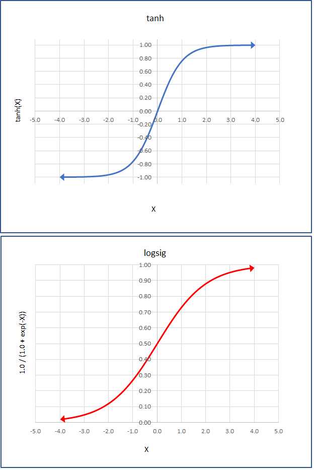
Figure 3-3: The Tanh and LogSig Activation Functions

In practice, for relatively simple neural networks, both activation functions usually give similar results, but tanh is used a bit more often than sigmoid for hidden layer activation. Other, less-common activation functions supported by CNTK include softplus, relu (rectified linear unit), leaky_relu, param_relu (parametric relu), and selu (scaled exponential linear unit).

Encoding and normalization

Neural networks only work directly with numeric data. Non-numeric data must be encoded. Numeric data should often be normalized (also called scaled) so that the magnitudes of the values are roughly the same. Suppose you have some training data that looks like:

27  42,000.00  liberal
56  68,000.00  conservative
37  94,000.00  moderate

The goal is to predict political leaning from a person’s age and income. You should normalize the age and income predictor values so that the relatively large incomes don’t swamp the ages. There are three common normalization techniques. The first technique, which doesn’t have a standard name, is to just multiply or divide all values by an appropriate power of 10. For example, you could divide all age values by 10, and all income values by 10,000:

2.7  4.20  liberal
5.6  6.80  conservative
3.7  9.40  moderate

Another technique is called min-max normalization. For each predictor variable, you replace a value with (max - value) / (max - min). For example, for the three raw age values, the max = 56 and the min = 27. The normalized age value for 37 is (37 - 27) / (56 - 27) = 0.3448. The min-max normalized data would be:

0.0000  1.0000  liberal
1.0000  0.5000  conservative
0.3448  0.0000  moderate

Using min-max normalization, all normalized values will be between 0.0 and 1.0 where a 0.0 is the normalized value for the smallest raw value, and a 1.0 is the largest value.

A third technique is called z-score (or Gaussian or normal) normalization. For each predictor variable, you replace the value with (value - mean) / (std dev). For example, for the raw age values, the mean is 40.0 and the standard deviation is 12.03. The normalized age value for 37 is (37 - 40.0) / 12.03 = -0.2494. The z-score normalized data would be:

-1.0808  -1.2247  liberal
1.3303   0.0000  conservative 
-0.2494   1.2247  moderate

Using z-score normalization, normalized values with typically be between -10.0 and +10.0 where a positive value is one that greater than the mean, a negative value is smaller than the mean, and a 0.0 is the mean value.

As a rule of thumb, I use divide-by-power-of-10 normalization when all values of all predictor variables have the same order of magnitude, because the technique is simple and preserves the sign of the raw data. I use z-score normalization when the underlying data is likely to be Gaussian distributed. I use min-max normalization when I can’t use power-of-10 or z-score normalization.

There are several ways to encode non-numeric predictor/feature values, but just one standard way to encode non-numeric class label values. Suppose you have some training data like:

female  2.5  democrat     white
male    4.0  republican   red
female  3.1  democrat     silver
male    5.3  independent  black
male    2.9  democrat     silver  

The goal is to predict a person’s car color (black, red, silver, or white) from their sex (male or female), age, and political affiliation (democrat, republican, or independent). The most common way to encode non-numeric predictor values is to use what’s called 1-of-(N-1) encoding. For a predictor variable that can be just one of two possible values, you encode as -1 or +1.

The 1-of-(N-1) technique for a predictor variable that can be three or more values is best explained by example. For the political affiliation data shown previously, you’d encode democrat as (1, 0), encode republican as (0, 1), and encode independent as (-1, -1).

Suppose a predictor variable can be one of five categorical values from a survey: terrible, weak, average, good, and excellent. You could encode terrible = (1, 0, 0, 0), weak = (0, 1, 0, 0), average = (0, 0, 1, 0), good = (0, 0, 0, 1), excellent = (-1, -1, -1, -1). In general, to encode a categorical variable that can take one of N values, you use N-1 values, where one value is a 1 and the other values are 0, except for the last categorical value which you encode as all -1 values.

Encoding a non-numeric class label (value to predict) is almost always done using what is called 1-of-N (also known as “one-hot”) encoding. If the class label can be one of three or more categorical values, you use N values where one value is a 1 and the other values are 0. For the data above where car color can be (black, red, silver, white), you could encode black = (1, 0, 0, 0), red = (0, 1, 0, 0), silver = (0, 0, 1, 0), and white = (0, 0, 0, 1).

The idea behind 1-of-N encoding is that you will design a neural network so that it outputs N values that sum to 1.0 and which can be interpreted as probabilities. Suppose an output is (0.20, 0.55, 0.15, 0.10) then because the largest probability is 0.55, the prediction maps to (0, 1 0, 0) which is the encoding for red.

To recap, if the original, raw car data is:

female  2.5  democrat     white
male    4.0  republican   red
female  3.1  democrat     silver
male    5.3  independent  black
male    2.9  democrat     silver  

Then the encoded data would be:

 1  2.5   1  0   0 0 0 1
-1  4.0   0  1   0 1 0 0
1  3.1   1  0   0 0 1 0
-1  5.3  -1 -1   1 0 0 0
-1  2.9   1  0   0 0 1 0

A special case occurs when the value to predict is binary. You can encode normally using (1, 0) and (0, 1), or you can encode as a single value that’s either 0 or 1. Binary classification and the two types of encoding the class label values are discussed in Chapter 5.

Normalizing and encoding training data is often time consuming and annoying. The CNTK library does not have any built-in normalization and encoding functions. Libraries such as pandas (“panel data” library) and scikit-learn (“science kit machine learning”) do have such functions, but those libraries have non-trivial learning curves. Typically, you must use a variety of techniques for data preprocessing.

Squared error and cross-entropy error

You can think of a neural network as a complex math function. The behavior of a neural network is determined by its input values, its weights and bias values, and its activation functions. Determining the values of the weights and biases is called training the network. The idea is to use a set of training data that has known input values, and known, correct output values, and then use some algorithm to find values of the weights and biases so that the error between computed output values, and the known correct output values, is minimized.

When using CNTK, you must specify which error metric to use, which learning algorithm to use, and how many training items to use at a time. The two most common forms of error metric for training are squared error and cross-entropy error (also called log loss). The demo program in Code Listing 3-2 shows how to compute squared error and cross-entropy error.

Code Listing 3-2: Squared Error and Cross-Entropy Error

The demo program first sets up four target items from a hypothetical training dataset:

targets = np.array([[1, 0, 0],
                    [0, 1, 0],
                    [0, 0, 1],
                    [1, 0, 0]], dtype=np.float32)

You can imagine this corresponds to four 1-of-N encoded class label items. Next, the demo sets up hypothetical associated raw (before softmax) computed output values:

computed = np.array([[7.0, 2.0, 1.0],
                     [1.0, 9.0, 6.0],
                     [2.0, 1.0, 5.0],
                     [4.0, 7.0, 3.0]], dtype=np.float32)

Notice that the row values do not sum to 1.0. Next, the demo applies softmax to the raw computed output values:

sm = C.ops.softmax(computed).eval()
print("\nSoftmax applied to computed = ")
print(sm)

The results are:

[[ 0.9909  0.0067  0.0025]
[ 0.0003  0.9523  0.0474]
[ 0.0466  0.0171  0.9362]
[ 0.0466  0.9362  0.0171]]

Notice that each row now sums to 1.0, and that the smallest-to-largest ordering is maintained. The demo program calculates both mean squared error and mean cross-entropy error from scratch, using just Python, and then using CNTK functions. The point is that in most situations you’ll want to use the built-in CNTK functions, but if you need a custom error metric, you can implement it without too much difficulty.

In order to understand the code, it’s useful to see how mean squared error and mean cross-entropy error are calculated by hand. The mean squared error could be calculated by hand as:

[ (0.9909 - 1)^2 + (0.0067 - 0)^2 + (0.0025 - 0)^2 +
  (0.0003 - 0)^2 + (0.9523 - 1)^2 + (0.0474 - 0)^2 +
  (0.0466 - 0)^2 + (0.0171 - 0)^2 + (0.9362 - 1)^2 +
  (0.0466 - 1)^2 + (0.9362 - 0)^2 + (0.0171 - 0)^2 ] / 4

= (0.0001 + 0.0045 + 0.0065 + 1.7857) / 4
= 1.7969 / 4
= 0.4492

In words, you compute the squared error for each item, add the squared error terms, and divide by the number of items. The demo prepares calculating mean squared error from scratch:

N = len(targets)  # 4
n = len(targets[0])  # 3

Then the demo walks through each row, using i as an index, and computes the squared error for the row as the sum of squared differences between the target values and the softmax values using j as an index. Then it accumulates the sum, and divides the accumulated sum by 4:

sum_se = 0.0
for i in range(N):  # each item
  for j in range(n):
    err = (sm[i,j] - targets[i,j]) * (sm[i,j] - targets[i,j])
    sum_se += err  # accumulate
mean_se = sum_se / N
print("\nMean squared error from scratch = %0.4f" % mean_se)

The output of this part of the demo program matches the result calculated by hand:

Mean squared error from scratch = 0.4492

Notice that if all softmax output values exactly equal the target values, mean squared error will be zero. The largest possible squared error for an item is 1.0, and therefore, the largest possible mean squared error for a set of items is 1.0. Next, the demo program calculates mean squared error using the built-in CNTK squared_error() function, like this:

mean_se = C.losses.squared_error(sm, targets).eval() / 4.0
print("\nMean squared error from CNTK = %0.4f" % mean_se)

As you’d expect, the output matches the previous computation and output:

Mean squared error from CNTK = 0.4492

Notice that squared_error() can operate on the full matrices rather than a row at a time, and that because squared_error() is type CNTK Function, you have to call the eval() function.

The squared error can be calculated for any two vectors of the same length. Cross entropy is a specialized form of error that applies only to two sets of probabilities, in other words, two vectors that have the same length, and that have values that sum to 1.0. If you have a set of predicted probabilities and a set of actual probabilities, the cross-entropy error is calculated as the negative of the sum of the products of the log of the predicted times the actual.

For example, suppose a set of predicted probabilities is (0.10, 0.60, 0.30), and the corresponding set of actual probabilities is (0.15, 0.50, 0.35). The cross-entropy error is:

CEE = - [ log(0.10) * 0.15 + log(0.60) * 0.50 + log(0.30) * 0.35 ]
        = - ( -0.3453 + -0.2554 + -0.4214 )
        = 1.0222

In classification problems, the softmax output values will sum to 1.0 and can be interpreted as probabilities, and a target vector will consist of one 1 value, and the rest 0 values, so it too can be interpreted as a probability set. For example, the first softmax item in the demo program is (0.9909, 0.0067, 0.0025), and the corresponding target vector is (1, 0, 0). Cross-entropy error is:

CEE = - [ log(0.9909) * 1 + log(0.0067) * 0 + log(0.0025) * 0 ]
        = - ( -0.0091 + 0 + 0 )
        = 0.0091

Notice that for classification problems, all but one term of the cross-entropy error will drop out. The demo program computes the cross-entropy error from scratch for the hypothetical classification data with these statements:

sum_cee = 0.0
for i in range(N):  # each item
  for j in range(n):
    err = -np.log(sm[i,j]) * targets[i,j]
    sum_cee += err  # accumulate
mean_cee = sum_cee / N
print("\nMean cross-entropy error w/ softmax from scratch = %0.4f" % mean_cee)  

The demo code follows the hand calculation closely. The output is:

Mean cross-entropy error w/ softmax from scratch = 0.7975

The demo program computes mean cross-entropy error in a slightly different way:

sum_cee = 0.0
for i in range(N):  # each item
  err = C.losses.cross_entropy_with_softmax(computed[i].reshape(1,3), \
    targets[i].reshape(1,3)).eval()
  sum_cee += err
mean_cee = sum_cee / N
print("\nMean cross-entropy error w/ softmax from CNTK = %0.4f" % mean_cee)

The output is:

Mean cross-entropy error w/ softmax from CNTK = 0.7975

Unlike squared_error(), which can easily compute over multiple items (in a matrix), cross_entropy_with_softmax() works more easily with one item at a time. Additionally, and somewhat surprisingly, CNTK v2.3 does not have a plain, cross-entropy error function—there’s only cross_entropy_with_softmax(). This means the function expects raw, pre-softmax values. Notice the function accepts computed rather than sm.

The reshape() function is a required detail. Because computed is a 4´3 matrix, computed[i] is the ith row which is an array. The cross_entropy_with_softmax() function requires a matrix, so, the array is cast to a 1´3 matrix.

To summarize, when you train a CNTK model you must specify which error function to use. The two main options are squared_error() and cross_entropy_with_softmax(). For classification problems with three or more class labels, either error function can be used, but cross_entropy_with_softmax() is recommended. For binary classification problems, if you set up a model with a single output node, you should use the special binary_cross_entropy() function, but if you set up a model with two output nodes, cross_entropy_with_softmax() is recommended. If you do use crosss_entropy_with_softmax(), you must remember not to explicitly apply softmax so that it isn’t applied twice. For all regression problems, squared_error() is recommended.

Stochastic gradient descent

Suppose you are training a model, and one of the weights currently has a value of 2.58. For a given training data item, you feed the input values to the model and compute the output values. Then you use an error function to determine something called the gradient, which is a number that indicates how far off, and in what direction, the computed output value is compared to the known correct output value. Suppose the gradient is +1.84. If you adjust (usually by subtraction) the weight by a fraction, called the learning rate (often indicated by Greek letter eta which looks like a script lower case “n”) then the computed output values will become slightly closer to the target output values. Suppose the learning rate is 0.01, then the new weight value is 2.58 - (1.84)(0.01) = 2.58 - 0.0184 = 2.5616.

Stochastic gradient descent is a complex topic, but CNTK handles most of the details for you. Typical CNTK code looks like:

batch_size = 10
learn_rate = 0.01
learner = C.sgd(nnet.parameters, learn_rate)
trainer = C.Trainer(nnet, (tr_loss, tr_clas), [learner])
. . .
curr_batch = rdr.next_minibatch(batch_size, input_map=my_input_map)
trainer.train_minibatch(curr_batch)

When stochastic gradient descent is used to train a neural network, the technique is often called back-propagation. In addition to the basic sgd() function, CNTK has several advanced variations, including adam() (“adaptive moment estimation”), and rmsprop() (“root mean squared propagation”).

When using any form of stochastic gradient descent, you must choose between online training (update weights after processing one training data item), batch training (update weights after processing all training items), or mini-batch training (update weights after processing a subset of all training items). In high-level pseudo-code, online training is:

loop max_iterations times
  for-each training item
    compute output values
    compute gradients
    use gradients to update each weight and bias value
  end-for
end-loop

In pseudo-code, batch training is:

loop max_iterations times
  set all accumulated_gradients = 0
  for-each training item
    compute output values
    compute gradients
    accumulate gradients
  end-for
  use accumulated gradients to update each weight and bias value
end-loop

In the early days of neural networks, batch training was most often used. Then online training became more common. Currently, mini-batch training is most often used. The CNTK library functions make it easy for you to try all three approaches.

Setting a value for the learning rate is mostly a matter of trial and error. A very small learning rate can make training very, very slow. A too-large learning rate can make training fail entirely. One technique for dealing with the learning rate magnitude problem is called momentum. Using momentum adds a boost to each weight update. What this means is you can use a relatively small learning rate, and the rate will effectively increase automatically for you. CNTK has a momentum_sgd() function for basic momentum, and a nesterov() function, which is an advanced version of momentum.

In the previous pseudo-code example, notice that training is an iterative process. You might guess that the more training iterations you can perform, the better. However, this is not always the case. If you over-train a model, you might get model overfitting. This is a situation where you have very low error (and high accuracy for a classification model) on the training data, but when presented with new, previously unseen data, your model predicts poorly.

There are several ways to reduce the likelihood of overfitting. As it turns out, overfitting is often associated with weights and bias values that have large magnitudes. Regularization is a technique that limits the magnitudes of weights and biases. There are two main forms of regularization, named L1 and L2. L1 regularization tends to lead to some weight values that are close to zero (effectively dropping their associated input nodes), and L2 regularization tends to lead to all weights and bias values being small, but few very close to zero. You can supply L1 or L2 regularization information as a parameter, for example:

learner = C.sgd(nnet.parameters, learn_rate, l2_regularization_weight=0.10)

Another technique used to limit overfitting is called train-validate-test. Using normal train-test, you divide all available training data into a training set (typically about 80% of available data items) and a test set (the remaining 20%). You use the training data to train your model, then feed the test dataset to the trained model. The accuracy of the trained model on the test data is a very rough estimate of the accuracy you can expect on new, previously unseen data.

With the train-validate-test technique, you divide all available training data into three sets: a training set (usually about 80% of the items), a validation set (10% of the items), and a test set (10% of the items). You train your model using the training dataset, but every few training iterations, you feed the validation data to the model. At some point, the error on the validation data may start to increase rather than decrease, indicating that model overfitting may be occurring. You can stop training, then evaluate the model on the test data. The train-validate-test technique is a meta-heuristic, not a well-defined algorithm. CNTK does not have any built-in functions that directly support train-validate-test.

The CNTK library organization

Technically, CNTK is a Python package. CNTK is organized into 13 high-level sub-packages and eight sub-modules (smaller sub-packages). The 10 most frequently-used of these are shown in Table 3-1.

Table 3-1: Most Important CNTK Packages

Notice that some function names appear in more than one package; for example, both the cntk.random and cntk.initializer packages have normal() and uniform() functions. These duplications are relatively rare, and in practice you shouldn’t have any trouble distinguishing between duplicate function names.

When writing CNTK with Python code, your indispensable resource is the API documentation. Because CNTK v2 is so new, there are relatively few good code examples available online. However, this will change as the use of CNTK increases.

Writing CNTK code is not easy, and you’ll run into problems. When I get an error, as a general rule of thumb, my first action is to determine the type of the offending object(s), for example:

t = type(foo)
print(t)

Then I’ll look up that type in the API reference. One of the most common sources of errors in CNTK programs is an incorrect shape of a matrix or array. Most CNTK objects are NumPy multidimensional arrays. You can use the NumPy shape property to determine an object’s shape, for example:

shp = foo.shape
print(shp)

In some rare situations, you may need to change the shape of an object. To do so, you can use the NumPy reshape() function. Note: throughout this e-book, I use the terms function and method, and the terms variable and object, more or less interchangeably.

Exercise

Using the program in Code Listing 3-1 as a guide, write a CNTK program that creates a 3-2-4 neural network with logistic sigmoid hidden layer activation and softmax output layer activation. Set the input-to-hidden weights to:

[[0.01, 0.02],
[0.03, 0.04],
[0.05, 0.06]]

Set the hidden-to-output weights to:

[[0.07, 0.08, 0.09, 0.10],
[0.11, 0.12, 0.13, 0.14]]

Set the hidden node bias values to [0.15, 0.16] and the output node bias values to [0.17, 0.18, 0.19, 0.20].

Compute the output values for input values = [2.0, 4.0, 6.0].

Answer: [0.2414, 0.2470, 0.2528, 0.2588]