Data Modeling with Cassandra and CQL

---

If you are coming from the relational world, it will take some time for you to get used to the many ways problems are solved in Cassandra. The hardest thing to let go of is data normalization. In the relational world, data is split into multiple tables so that the data has very little redundancy. The data is logically grouped and stored, and if we need a certain view on this data, we make a query and present the desired data to the user.

With Cassandra the story is a bit different. We have to think about how our data is going to be queried from the start. This causes a lot of write commands to the database because data is often inserted into multiple tables every time we store something in Cassandra. One of the first thoughts that may come to mind here is that this is not going to be responsive or fast, but remember, Cassandra is really fast at writing.

Another concern you may have is that this will probably store a lot more data than we actually need, and you are right about that; Cassandra will probably store a lot more data on the disk than a relational database will. This heavy writing pays off when running queries because the queries are already prepared and there is no complex, time-consuming data joining. The entire Cassandra philosophy could be summarized with the premise that the disk is cheap.

Comparing Relational and Cassandra Data Storage

To compare classical relational storage and Cassandra, we need to start with the model. As an example, we’ll use an online used car market. Let’s start with the relational data model.

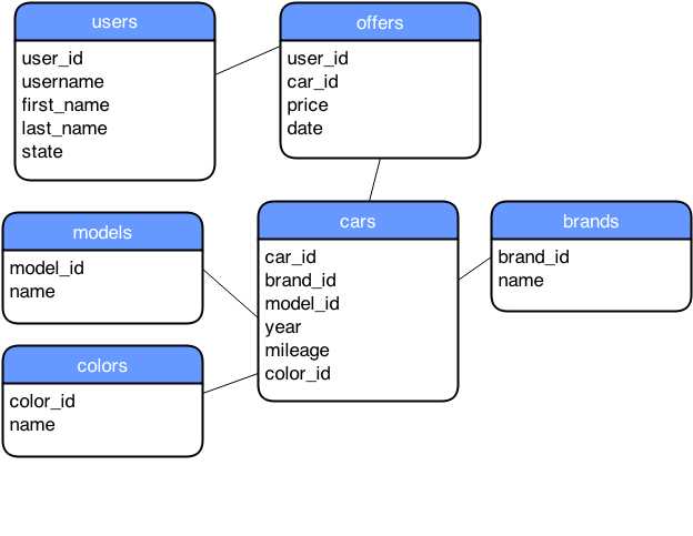
35. Simple relational model of an online car market

Figure 35 shows a simple relational model for an online used car market. Every box in the figure would become a separate table in a relational database. Elements inside the boxes would become columns in the tables. Every stored row would have each column defined in the model saved to the disk. If the creator of the table specifies it, the columns can have an undefined or a null value, but they would still be stored on the disk. When relational data from the model in Figure 35 is stored, it might look something like the following figure.

36. Example of stored relational data

To examine Cassandra’s way of storing data, we first have to look at how the data is actually structured.

37. Cassandra Data Structuring

We already talked about the keyspace and the column family. Column family is also often simply called a table. A row in Cassandra can have all of the columns defined or just some of them. Cassandra will save only actual values to the row. Cassandra’s limitation for a row is that it must fit on a single node. The second limitation for a row is that it can have at most two billion columns. In most cases, this is more than enough, and if you exceed that number, the data model you defined probably needs some tweaking.

The previous figure shows columns in a row storing a value and a time stamp. The columns are always sorted within a row by the column name. We’ll discuss how to model the example of the used car market with Cassandra in the next sections, but for now, let’s just show how the user’s table would be stored in Cassandra. Note that we didn’t use an auto-increment key as is often the case with relational data modeling; rather, we used a natural key username. For now, let’s skip the CQL stuff and just look at the stored data at an abstract level:

38. Cassandra storing example user data

The previous figure shows the low-level, data-storing technique Cassandra uses. The example is pretty similar to the way the relational database stores data. Now, let’s look at the way the data is stored if the row keys were the states and the clustering columns were the usernames. Also, let’s add John Q. Public to NY to illustrate the difference.

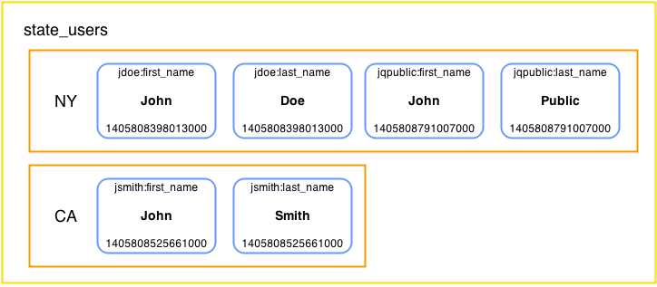
39. Cassandra storing example user data with state as partition key

The data storage in the previous figure might seem a little strange at the moment because column names are fairly fixed in relational database storage systems. It uses a username to group the columns belonging to a single user into a group. Remember, columns are always sorted by their names. Also note that there is no column for the username and that it’s stored only in the column name. However, this approach to storage does not allow direct fetching of users by their username. To access any of the data contained within the row (partition), we need to provide a state name.

Now that we know how Cassandra is handling the data internally, let’s try it in practice. By now, we have talked about a lot of Cassandra concepts and how they differ from relational databases. In the next section, we’ll dive into the CQL, the language used for interacting with Cassandra.

CQL

CQL, or Cassandra Query Language, is not the only way of interacting with Cassandra. Not long ago, Thrift API was the main way of interacting with it. The usage, organization, and syntax of this API were oriented toward exposing the internal mechanisms of Cassandra storage directly to the user.

CQL is the officially recommended way to interact with Cassandra. The current version of CQL is CQL3. CQL3 was a major update from CQL2. It added CREATE TABLE syntax to allow multicolumn primary keys, comparison operators in WHERE clauses on columns besides the partition key, ORDER BY syntax, and more. The main difference from standard SQL is that CQL does not support joins or subqueries. One of the main goals of CQL is, in fact, giving users the familiar feeling of working with SQL.

CQL Shell

In the previous chapter we looked at how to install and run DataStax DevCenter. If you don’t want to use the DataStax DevCenter, go to the directory where you installed Cassandra, and then go to the bin directory and run the cqlsh utility.

Code Listing 3

After running the CQL shell, you can start issuing instructions to Cassandra. The CQL shell is fine for most of the day-to-day work with Cassandra. In fact, it is the admin’s preferred tool because of its command-line nature and availability. Remember, it comes bundled with Cassandra. DevCenter is more for developing complex scripts and developer efficiency.

Keyspace

Before doing any work with the tables in Cassandra, we have to create a container for them, otherwise known as a keyspace. One of the main uses for keyspaces is defining a replication mechanism for a group of tables. We’ll start by defining a keyspace for our used car market example.

Code Listing 4

When creating a keyspace, we have to specify the replication. Two components defining the replication are class and replication_factor. In our example, we have used SimpleStrategy for the class option; it replicates the data to the next node on the ring without any network-aware mechanisms.

At the moment, we are in the development environment with only one node in the cluster so a replication factor of one is sufficient. In fact, if we specified a higher replication factor—3, for instance—and then used the quorum option when performing selects, the select commands would fail because quorum cannot be reached with a replication factor 3 because 2 nodes have to respond, and we have only one node in our cluster at the moment. If we added more nodes to the cluster and would like the data to be replicated, we can update the replication factor with the ALTER KEYSPACE command as shown in the following code example.

Code Listing 5

SimpleStrategy will not be enough in some cases. The first chapter mentioned that Cassandra uses a component called snitch to determine the network topology and then uses different replication mechanisms that are network-aware. To enable this behavior on the keyspace, we have to use the NetworkTopologyStrategy replication class, as shown in the following example.

Code Listing 6

The previous example replicates the used_cars keyspace with replication factor 1 in DC1 and replication factor 3 in DC2. Data center names DC1 and DC2 are defined in node configuration files. We don’t have any data centers specified in our current environment but the command will still run and create a keyspace with the options that we specified.

On some occasions, we will need to delete the complete keyspace. This is achieved with the DROP KEYSPACE command. The command is pretty simple and has only one parameter: the name of the keyspace that we want to delete. Keyspace removal is irreversible and issuing the command causes immediate removal of the keyspace and all of its column families and their data.

Code Listing 7

The DROP KEYSPACE command is primarily used in development scenarios, migration scenarios, or both. If you drop a keyspace, the data is removed from the system and can only be restored from a backup.

When issuing commands in the CQL shell, we usually have to provide a keyspace and table. The following SELECT command lists all users in the used_cars keyspace.

Code Listing 8

This becomes a bit tedious over time, and most of the operations issued in sequence are usually within a single keyspace. So, to reduce the writing overhead, we can issue the USE command.

Code Listing 9

After running the USE command, all of the subsequent queries are run within the specified keyspace. This makes writing queries a bit easier.

Table

Defining and creating tables is the foundation for building any application. Although the syntax of CQL is similar to SQL, there are important differences when creating tables. Let’s start with the most basic table for storing users.

Code Listing 10

PRIMARY KEY is required when defining a table. It can have one or more component columns, but it cannot be a counter column. If the PRIMARY KEY consists of only one column, you can place PRIMARY KEY into the column definition after specifying the column type.

Code Listing 11

If we were using SQL and a relational database to specify columns in the PRIMARY KEY, all of the columns would be treated the same. In the previous chapter we discussed how Cassandra stores data, and that all data is saved in wide rows. Each row is identified by an ID. In Cassandra terminology, this ID is called the partition key. The partition key is the first column from the list of columns in the PRIMARY KEY definition.

Note: The first column in the PRIMARY KEY list is the partition (row) key.

Let’s use an example to see what is going on with the columns specified after the first place in the PRIMARY KEY list. We will model the offers shown when we compared relational and Cassandra data storage. We mentioned earlier that normalization is not common when working with Cassandra. The relational example we used stored the data about car offerings into five tables. Here, we are going to use just one table, at least for now.

Code Listing 12

The PRIMARY KEY definition consists of two columns. The first column in the list is the partition key. All of the subsequent listed columns after the partition key are clustering keys. The clustering keys influence how Cassandra is organizing the data on the storage level. To keep things simple, we’ll just concentrate on brand and color to show what the clustering key does. The table with offers might look something like the following when queried.

Code Listing 13

This looks pretty similar to what we would expect from a table in relational storage.

When it comes down to physically storing the data, the situation is a bit different. The clustering key date is combined with the names of the other columns. This causes the offers to be sorted by date within the row.

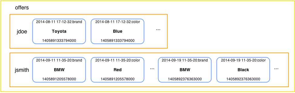
40. Cassandra storing offers data with date as clustering key

Now the question is, what would happen if we didn’t add date to the second place in the PRIMARY KEY list, causing it to become a clustering key? If you look more carefully, the column names in the previous figure are combinations of date and column names such as brand and color. If we removed date as a clustering key, every user would have just one used car offer and that’s it. date would become just another column and we would lose the possibility to add more offers per user.

Sometimes data will be too large for a single row. In that case, we combine the row ID with other data to split the data further into smaller chunks. For instance, if our site became mega popular and if all car retailers offered their cars on our site, we would somehow have to split the data. Perhaps the most reasonable way to do it would be to split the data by the car brand.

Code Listing 14

Note that if a row is a combination of username and brand, we will be unable to access the offers without specifying the username and brand when fetching the row. Sometimes when such a technique is used, the application has to combine the data to present it to the user. A partition (row) key that consists of more than one column is called a composite partition key. A composite partition key is defined by listing the columns in parentheses. Remember, only the first column in the list is the partition key. If we want more columns to go into the partition key, we have to put them in parentheses.

CQL Data Types

At this point we have used different types to specify column data but have yet to discuss them. The following table provides a short overview of the data types in Cassandra.

1. CQL Data Types

The column type is defined by specifying it after the column name. Changing column type is possible if the types are compatible. If the types are not compatible, the query will return an error. Also note that the application might stop functioning because the types may not be compatible on the application level. Changing the clustering column or columns that have indexes defined on them is not possible. For instance, changing the year column type from int to text is not allowed and causes the following error.

Code Listing 15

Adding columns to Cassandra tables is a common and standard operation.

Code Listing 16

The previous code listing adds an integer type column called airbags to the table. In our example this column stores the number of airbags the vehicle has. Dropping the column is done with the DROP subcommand from the ALTER TABLE command.

Code Listing 17

To complete the life cycle of a table, we have to run two more commands. The first is for emptying all of the data from the table.

Code Listing 18

The final command is for dropping the entire table.

Code Listing 19

Table Properties

Besides column names and types, CQL can also be used to set up the properties of a table. Some properties such as comments are used for easier maintenance and development, and some go really deep into the inner workings of Cassandra.

2. CQL Table Properties

Defining tables with comments is pretty easy and represents a positive practice for maintenance and administration of the database.

Code Listing 20

Most of the options are simple to define. Adding a comment is a nice example of such an option. On the other hand, compression and compaction options have subproperties. Defining the subproperties is done with the help of a JSON-like syntax. We’ll look at an example shortly.

3. CQL Table Compression Options

Manipulating compression options can lead to significant performance gains, and many Cassandra solutions out there run with compression options set to non-default values. Indeed, tuned compression options are sometimes very important for a successful Cassandra deployment, but most of the time, especially if you are just starting to use Apache Cassandra, you will be just fine using the default SnappyCompressor settings as the compression option.

Compaction has many subproperties as well.

4. CQL Table Compaction Options

The options for compression and compaction options are defined with JSON-like syntax.

Code Listing 21

Cluster Ordering the Data

Previously we noted that columns within a row on the disk are sorted. When fetching the data from physical rows in the table, we get the data presorted by the specified clustering keys. If the data is, by default, in ascending order, then fetching in descending order causes performance issues over time. To prevent this from happening, we can instruct Cassandra to keep the data in a row of a table in descending order with CLUSTERING ORDER BY.

Code Listing 22

It is important to remember that the previous CREATE TABLE example keeps the data sorted in descending order but only within the row. This means that selecting the data from a specific user row with a username will show sorted data for that user, but if you select all the data from the table without providing the row key (username), the data will not be sorted by username.

Tip: Clustering sorts the data within the partition, not the partitions.

But just to remember all this even better, let’s consider an example. Let’s go back to our offers table. The offers table is sorted in ascending order by default, but this is fine for demonstrating what the previous tip is all about. First, we’ll select the offers for the jsmith user.

Code Listing 23

Notice that these offers are sorted in ascending order, with the oldest record being in the first place. And that’s what we would expect if the data were sorted by date since this column is the clustering key. But some Cassandra users may be confused when they try to access the whole table without providing the row key (username):

Code Listing 24

Notice that the data has no sorting whatsoever by the username (row ID, partition key) column. Once again, the data is sorted within a username but not between usernames.

Manipulating the Data

Up until now, we have been concentrating mostly on the data structure and the various options and techniques for organizing stored data. We covered the basic data reading but we’ll look at more advanced examples of data retrieval soon. Inserting data looks pretty much like it does in standard SQL databases; we define the table name and the columns and then specify the values. One of the simplest examples is entering data into the users table.

Code Listing 25

The previous code shows you how to insert data into the users table. It has only text columns so all of the inserted values are strings. A more complex example would be to insert values into the offers table, as in the following example.

Code Listing 26

Working with strings and numbers is pretty straightforward. Numbers are more or less simple; the decimal separator is always a period because insert parameters are split with a comma. A number cannot begin with a plus sign, only a minus sign. The numbers can also be entered with scientific notation, so both “e” and “E” are valid when specifying a floating-point number. Note that DataStax DevCenter marks numbers defined with an “e” as incorrect syntax usage, while the CQL shell interprets both signs as valid. After the “e” that specifies the exponent, a plus or minus sign can follow. The following code example inserts a car that costs $8,000 specified in scientific notation with a negative exponent prefix.

Code Listing 27

Strings are always placed inside single quotation marks. If you need the single quotation mark in the data, escape it with another single quotation mark before placing it in the string as in the following example.

Code Listing 28

Besides numbers and strings, the previous queries also contain dates. Dates are defined as the timestamp type in Cassandra. A timestamp can simply be entered as an integer, representing the number of milliseconds that have passed since January 1, 1970 at 00:00:00 GMT. The string literals for entering timestamp data in Cassandra are entered in the following formats.

5. Timestamp String Literal Formats

The format is pretty standard in many programming languages and database environments. Besides using a space to separate the date and time parts, sometimes they are separated with a T. The time zone is specified in a four-digit format and is noted with the letter Z in the format examples in the previous table. The time zone can begin with a plus or a minus sign, depending on the position of the time zone compared to GMT (Greenwich Mean Time). The first two digits represent the difference in hours and the last two digits represent the difference in minutes.

Most time zones are an integer difference when compared to GMT. Some regions have an additional half hour offset, such as Sri Lanka, Afghanistan, Iran, Myanmar, Newfoundland, Venezuela, Nepal, the Chatham Islands, and some regions of Australia. If no time zone is specified, the time zone from the coordinator node is used. Most of the documentation recommends specifying the time zone instead of relying on the coordinator node time zone. If the time zone is not specified, it is assumed that you wanted to enter ’00:00:00’ as the time zone.

The default format for displaying timestamp values in the CQL shell is “yyyy-mm-dd HH:mm:ssZ”. This format shows all of the available information about the timestamp value to the user.

Sometimes you will want to update the data that has been written. As in standard SQL database systems, it is possible to update records, but the inner workings of the UPDATE command in Cassandra are a bit different. Let’s change the brand and the model of an offer that user jdoe made on 2014-08-11.

Code Listing 29

Updating the value actually adds a new column within the row with the new time stamp and marks the old columns with tombstones. The tombstone is not set immediately, the data is just written. With the first read or compaction process starts, Cassandra will compare the two columns. If the column names are the same, the one with a newer time stamp wins. The other columns are marked with tombstones. This is easier to visualize in the following figure.

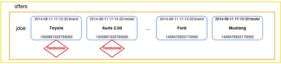
41. Updating columns: The old columns get tombstones, and new columns are added with new values

When manipulating data, there is another important difference when comparing Cassandra to SQL solutions. Let’s review the current table data.

Code Listing 30

Now, let’s try to insert the first offer from the jdoe user but with a different brand and model.

Code Listing 31

What do you think would be the result of the previous INSERT statement? Well, if this were a classical SQL database, we would probably get an error because the system already has data with the same username and date. Cassandra is a bit different. As mentioned before, INSERT adds new columns and that’s it. The new columns will have the same names as the old ones, but they will have new time stamps. So when reading the data, Cassandra will return the newest columns. After running the previous INSERT statement, running the same query as in Code Listing 30 would return the following.

Code Listing 32

On some occasions you will want to delete data. This is done with the DELETE statement. Usual SQL systems allow the DELETE statement to be called without specifying which rows to delete. This then deletes all the rows in the table. With Cassandra, you must provide the WHERE part of the DELETE statement for it to work, but there are some options. We can always specify just the partition key in the WHERE part. This removes the entire row and, in effect, all of the offers made by the user.

Code Listing 33

The previous statement is a rather dangerous one because it removes the entire row, and it is done with a username that is not present in our example. Usually, when deleting the data, all of the primary key columns are specified, not just the partition (first) key.

Code Listing 34

Data Manipulation Corner Cases

In the previous section, we used an INSERT statement using the same partition and clustering key with new data set in the columns instead of updating the row. This technique is called upserting.

Upserting is a very popular technique in Cassandra and is actually the recommended way to update data. It also makes system maintenance and implementation easier because we don’t have to design and implement additional update queries.

Tip: Upsert data by inserting new data with the old key whenever possible.

Upserting data is what you should be doing most of the time in Cassandra, but let’s compare it with inserting. Let’s assume that, for some reason, users can change all of the offers in our example at any time. We will analyze the fields and see what changes are even possible.

It would not be wise to let the system change the username on the offer. This would actually represent a serious security issue if left to any user. For our comparison, we’ll assume that the administrator of the system will be able to change the username. Let’s try changing it.

Code Listing 35

OK, this didn’t work but while we are at it, let’s try to change the offer date and set it to the day after the offer date with the UPDATE command. The date field is not a partition key. In actuality, it is a clustering key, so it might just work.

Code Listing 36

OK, this didn’t work either. date is also a part of the primary key. You may have expected it because of the error message received in the first try. Updating primary key columns is not possible.

This example is very important to remember. Cassandra does not allow updates to any of the primary key fields.

Note: Cassandra does not allow updates to primary key fields.

If you have some data that might require this kind of update, and if it is data that changes a lot, you might want to consider other storage technologies or move this logic to the application level. This could be done in two steps. The steps are interchangeable; the choice is left to the system designer. Let’s consider an example where the first step is to insert the new data and the second is to delete the old data.

Code Listing 37

The database will be in an inconsistent state before the DELETE statement is issued, but the situation would be the same if we reversed the steps. If the INSERT happens before the DELETE, two offers might be visible in the system for a while. If the DELETE happens before the INSERT, an offer might be missing. As mentioned before, it’s up to the system designers to decide which is lesser of the two evils.

The previous case will work just fine in most situations. Still, sometimes it’s possible due to various concurrency techniques that the previous queries won’t run in an order we intended for them. Issuing the previous commands from a shell or from DevCenter will always run in this order, but when the application issues multiple requests, it might lead to inconsistency.

Also, some systems might have clocks that are not 100 percent in sync. If, for instance, the clocks have offsets even in the milliseconds range, it is very important that the commands are issued exactly one after the other. Simply add USING TIMESTAMP <integer> to the statements that you want to run in a specific order. The Cassandra clusters will then use the provided USING TIMESTAMP instead of the time when they received the command. Using this option on an application level will, in most cases, prevent the caching of prepared statements, so use it wisely. Also, note that this option is usually not issued if users give the commands sequentially by typing.

Playing with the TIMESTAMP option might be a little tricky. For instance, if by some mistake we issue a DELETE that is in the future, we might work with an entry normally, and later wonder why it disappeared without having issued a DELETE command.

Anyway, the following code example issues the previous INSERT and DELETE statement combination with the TIMESTAMP option.

Code Listing 38

The INSERT statement has the TIMESTAMP option specified at the end. In the DELETE statement, it’s specified before the WHERE part of the statement. The TIMESTAMP option is rarely used, but it is included here because knowing about this option might save you some time when encountering weird issues when manipulating data in Cassandra.

Querying

So far, we’ve spent a lot of time exploring data manipulation because to work with queries, we have to create some data in the database. The command for retrieving data is called SELECT, and it has appeared in a couple of examples in previous sections of the book. For those of you with experience in classical SQL databases, you won’t have any problems adapting to the syntax of the command, but the behavior of the command will probably seem a bit strange. Remember, with Cassandra, the emphasis is on scalability.

There are two key differences when comparing CQL to SQL:

• No JOIN operations are supported.
• No aggregate functions are available other than COUNT.

With classical SQL solutions, it’s possible to join as many tables together as you like and then combine the data to produce various views. In Cassandra, joins are avoided because of scalability. It is a good practice for developers and architects think up-front about what they will want to query and then populate the tables accordingly during the write phase. This will cause a lot of data redundancy, but this is actually a common pattern with Cassandra. Also, we mentioned in a previous chapter that the disk is considered to be the cheapest resource when building applications with Cassandra.

The only allowed aggregate function is COUNT, and it is often used when implementing paging solutions. The important thing to remember with the COUNT function is that it won’t return an actual count value in some cases, and also that this function is restricted with a limit. The most common limit value is 10000, so if the expected count is larger but the function returns exactly 10000, you may need to increase the limit to get the exact value. At the same time, be very careful and bear in mind that this might cause performance issues.

In the previous sections, we discussed the basic SELECT statements and limited ourselves to displaying specific columns because not enough space was available to show all of the table columns nicely. Building the queries was easy because we knew the keyspace names, table names, and column names in the tables. DevCenter makes this easier because of the graphical interface, but for those of you using the CQL shell, the situation requires a couple of commands to find your way around. The most useful command is DESCRIBE. As soon as you connect to Cassandra with the CQL shell, you can issue the following command.

Code Listing 39

Now we see our used_car keyspace is available and we can issue the USE command on it. Now that we are in the used_cars keyspace, it would be nice if we could see what tables are available. We can use the DESCRIBE command with the tables parameter to do just that.

Code Listing 40

Using the DESCRIBE command with the tables parameter gave us a list of tables. Most of the tables in the previous listing are system tables; we usually won’t have any direct interaction with them through CQL. Now that we have a list of tables in the used_cars keyspace, it would be very interesting for us to see the columns in the table and their types. Let’s look it up for the offers table.

Code Listing 41

The most interesting result of the previous command is column names and their types. If you want to optimize and tweak the table behavior, you will probably use this command to check if a setting was successfully applied to the table. Let’s check the current state in the offers table.

Code Listing 42

It would be very interesting for us to see only the offers from a specific user. Since the user jsmith has the most offers, let’s concentrate on them. Picking their offers will be done with the WHERE clause and specifying the jsmith username.

Code Listing 43

You might want to filter the offers table for multiple users and build a query that would return all of the offers for users jsmith and adoe.

Code Listing 44

The OR operator does not exist in Cassandra. If we want to select multiple offers from the users, we have to use the IN operator.

Code Listing 45

We’ll concentrate on the offers from the jsmith user again and select the offer that the user made on a specific date. Remember, the offer is identified by the combination of the username and the date information for the offer. If you go back to the previous section, you will find that the username and date information form a primary key. The query is:

Code Listing 46

If we would like to get two specific orders for the user from the table, we could again use the IN operator as shown in the following example.

Code Listing 47

But listing all of the dates to get the offers from the user is not the most efficient way to query the data. Think about it; we would actually have to know every piece of data in the list in order to get the listing. A more practice-oriented query would be to show all of the offers made by the user since a certain time or all of the offers made within a period of time. Let’s look at the offers jsmith did in September.

Code Listing 48

Some might set the end date to be ‘2014-09-30’, but this would not return offers made on the last day of the month because CQL, by default, assumes the values for hours, minutes, and seconds are set to zero. So, specifying the 30^th would, in effect, ignore all of the offers after midnight, or in other words, all the offers for that day.

The simplest way to approach this is to specify the first day of the following month as the end date with the less than operator. The previous query is not 100 percent correct, actually. The offers made between the stroke of midnight and the expiration of the first millisecond will not be included in the results. To cover this case, simply add the equal sign after the greater-than sign. The comparison operators are not always possible in Cassandra. Cassandra will allow comparison operators only in the situations where it can retrieve data sequentially.

In previous examples, all of the offers from the user are automatically sorted by their date by Cassandra. That’s why we could use the greater-than and less-than operators. We did this on the clustering part of the primary key. Now, just for a moment, let’s take a small step back and try some sort of comparison with the first part of the primary key. We will create a whole new table to do that, just to show the situation for the numbers:

Code Listing 49

As the previous error message says, the first part of the primary key can only be retrieved with the equal sign and an IN operator. This is one of Cassandra’s limitations when it comes to querying the data. Let’s look into the other parts of the primary key. We will create a new and independent example to show Cassandra’s behavior in this case.

Code Listing 50

The previous results look just fine. We specified what row we wanted to read and provided the range. Cassandra can find the row, do the sequential read of it, and then return it to us. This is possible because the values from column b actually become columns. So, in row A we don’t have columns called b, but we have columns called 1:c, 2:c, etc., and the values in those columns are A1, A2, etc.

I’m reviewing how Cassandra stores tables because it is very important to understand the internals of Cassandra in order to use them as efficiently as possible.

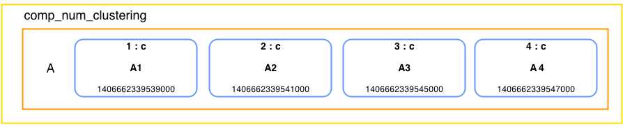
42. Cassandra storage of the table in Code Listing 50

Everything is fine with the ranges, but what would happen if we tried this on multiple rows? What if we wanted all of the data where b is greater than some number, let’s say, 3?

Code Listing 51

This might seem a bit unexpected, especially to people coming from the relational world. The numbers are ordered so why we are not getting all of the data out? Well, the previous table might have multiple rows. In order to find all the data, the client would have to potentially contact other nodes, wait for their results, go through every row that it receives, and then read the data out of them. This simple query could very easily contact every node in the cluster and cause serious performance degradation. In Cassandra, everything is oriented toward performance. So, that kind of querying is not possible out of the box or even allowed in some cases. One way of making this kind of querying possible is with the ALLOW FILTERING option. The following query would return the results just as we might expect them.

Code Listing 52

ALLOW FILTERING will let you run some queries that might require filtering. Use this option with extreme caution. It significantly degrades performance and should be avoided in production environments. The main disadvantage of the filtering is that it usually involves a lot of queries to other nodes and, if done on big tables, it may cause very long processing times that are pretty nondeterministic. While we are at it, let’s try the filtering option for column c.

Code Listing 53

Indexes

The filtering option does not give us the ability to search the table by the data in the c column. The error message warns us that there are no indexed columns, so let’s create an index in the table for the c column.

Code Listing 54

The previous query returned the results once we created the index on the column. Creating indexes might seem the easy way to add searching capabilities to Cassandra. Theoretically, we could create an index on the table any time we needed to search for any kind of data, but creating indexes has some potentially dangerous downsides.

Cassandra stores the indexes just as it stores the other tables. The indexed value becomes the partition key. Usually, the more unique values there are, the better the index performance. On the other hand, maintaining this index will be a significant overhead for the system if the number of rows grows because every node will have to have most of the information that the other nodes store. The other possibility is that we have some binary index with some sort of true-false values. This would be an index with a very small number of unique values. That kind of index quickly gets many columns in just a couple of rows and becomes unresponsive over time because it is searching within the two very large rows. One important point is that if the node fails and we restore the data, the index will have to be rebuilt from scratch. As a rule of thumb, the best use for indexes is on relatively small tables with queries that return results in tens or hundreds but not more.

The index that we created in the previous example returned an automatic name because we simply forgot to specify a name for it. This is a very common mistake. Indexes are updated on every write to Cassandra and there are techniques that eliminate the need for them, so if we at some point in time decide to remove the index, we will run into trouble because we have to know its name in order to remove it. The following query makes it possible for us to find the index name together with other information that is relevant for identifying it.

Code Listing 55

We have made an index in the c column of the comp_num_clustering table, so the index that we are looking for must be the last index in the table shown after running the previous query. The following example shows how to remove the index.

Code Listing 56

The previous index name seems pretty reasonable, and from the name we can determine what this index is all about. If you don’t like the naming Cassandra does automatically, or you have some special naming convention that you have to enforce, then you can do name the index with the following command.

Code Listing 57

This way, you can keep the index name in the initialization scripts for other nodes or development environments and avoid depending on the automatic index naming that might change in future versions of Cassandra.

Now that you know how Cassandra fetches data and that it’s not always possible to get data with any column value out, let’s look at the ORDER BY clause. Using this clause is not always possible. Most relational databases allow combinations of multiple columns on almost all queries. Cassandra limits this for performance gains. ORDER BY can be specified on one column only, and that column has to be the second key from the primary key specification. On the comp_num_clustering table, it’s the b column; in the offers, it is the date column. Two possible orders are ASC and DESC. As an example, we will reverse the jsmith user’s offers in time and put them in descending order. They are ascending by default because Cassandra sorts by column names, so there is no need to use ASC on the offers table.

Code Listing 58

ORDER BY is not used often. It’s more common to specify the clustering option when creating the table so that the data is automatically retrieved in the order that the system designers intended it. Most of the time, ordering is based on some kind of time-based column like a sensor, user activity, weather, or some other readings.

Collections

The primary use for collections in Cassandra is storing a small amount of denormalized data together with the basic set of information. The most common usages for collections are storing e-mails, storing properties of device readings, storing properties of events that are variable from occurrence to occurrence, and so on. Cassandra limits the amount of elements in a collection to 65,535 entries. You can insert data past this limit but the data is preserved and managed by Cassandra only up to the limit. There are three basic collection types:

• map
• set
• list

These structures are pretty common in most programming languages today, and most readers will have at least a basic understanding of them. We’ll show each structure with a couple of examples, and while we’re at it, we’ll expand our data model a bit and make use of the collections.

We’ll start with the map collection in our used car example. By now, we have defined the offers table and specified some basic offer attributes such as date, brand, color, mileage, model, price, and year. Now, we know that different cars have very different accessories in them. Some cars might run on different fuels, have different transmissions, or have different numbers of doors. We could cover all these extra properties without adding new columns to our offers table if we specified a map type column in the offers table as shown in the following example.

Code Listing 59

Now that we have the equipment map on our offers, let’s talk a bit about the properties of the map collection. Long story short, a map is a typed set of key-value pairs. The keys in the map are always unique. One interesting property of the values in a map when stored in Cassandra is that the keys are always sorted.

There are two ways to define map key-value pairs. One is to update just the specific key in the map. The other is to define a whole map at once. Both ways are possible with the UPDATE command, but when using INSERT, you can specify just the whole map. Let’s see what an INSERT would look like.

Code Listing 60

The syntax for defining the maps is pretty similar to the very popular JSON format. The comma separates the key-value pairs and the key is separated from the value by a colon. The saved row looks like the following.

Code Listing 61

Notice that the stored map values are sorted and that they don’t depend on the order we defined them. If we ever decide to change the values in the map or add a new one without discarding the old values, we can use the following UPDATE commands.

Code Listing 62

The previous query will update the doors key in the map and will add a new turbo key to it. This syntax is used when doing updates because we don’t have to care if the key was created or not. We simply specify its value and Cassandra will update the key with the new value if it is able to find it, or it will define a new key if it’s unable to find it. Let’s see what the data looks like at the moment.

Code Listing 63

If we wanted to redefine the complete map, we would simply set equipment to be equal to a whole new map definition as it was done in Code Listing 60. Still, sometimes we will want to remove just specific keys from the map. This is done with the DELETE command.

Code Listing 64

Deleting a key that does not exist in the map is not a problem. You can run the previous example as many times as you like but it will delete the turbo key only on the first run. We have yet to cover the concept of time to live (TTL). For now, just remember that Cassandra can automatically delete data after it has lived for a specified period of time. For instance, if you insert or update a key-value with a time to live parameter, the time the data will actually live refers only to the changed, inserted key-value pair. All the other data have their own times to live. We will discuss the TTL concept more in depth later. For now, it’s enough to know that collections specify a TTL on an element level, not on the row or the column level.

The next collection type we are going to dive into is the set. A set is a collection of unique values. Cassandra always orders sets by their value. Creating a column that is a set is done with the set keyword followed by the type of key elements in angled brackets. One of the most common uses for sets is saving user contact data such as e-mail addresses and phone numbers. Let’s add a set of e-mails to the users table.

Code Listing 65

Now the users table can store more e-mails for every user. Inserting a new user is shown in the following example.

Code Listing 66

The difference in sets when compared to maps is that there are no key elements, there are just values. If you add duplicates in the previous e-mail list, the duplicated values will not be stored in Cassandra. The values in the set are always sorted just as the keys in maps are.

The updating syntax is based on the plus and minus operators. If we wanted to first remove an e-mail address from the set and then add a new one, we would do it with the following queries.

Code Listing 67

The previous queries result in the following emails for the user jqpublic.

Code Listing 68

The last collection type in Cassandra is a list. A list is a typed collection of non-unique values. The values in the list are ordered by their position. Map and set values are always sorted. The list elements always remain in the position where we put them. The most basic example would be a to-do list. We’ll show how to use the list in the next examples. Before doing anything with the list, we have to define one.

Code Listing 69

Maps and sets are set in braces, but the list is in brackets. Other than that, the list is pretty similar to the previous two collection types. Let’s see how to define a list when inserting data into a table.

Code Listing 70

The previous INSERT statement generated a simple to-do list for a user, with three elements in it. Let’s have a look at what’s in the table.

Code Listing 71

When referencing the elements in the list, we do so by their position. The first element in the list has the position 0, the second 1, and so on. The following example shows how to update the first element in the to-do list of the user.

Code Listing 72

In some situations, we will want to add elements to the list.

Code Listing 73

Cassandra can also remove occurrences of items from the list.

Code Listing 74

It’s also possible to delete elements with a specific index in the list.

Code Listing 75

All of the previous changes in the list should result in the following.

Code Listing 76

Now we know how to use collections in Cassandra. Collections are a relatively new concept in Cassandra. They are very useful in many day-to-day situations. Because they are very easy to work with, they might sometimes be overused. Be very careful and don’t fill up collection columns with data that might be in the tables. All of the collection types are limited to 65,535 elements; having more would definitely be a sign that you are doing something wrong.

Time Series Data in Cassandra

Knowing how something changes over time is always important. By having the historical data about some kind of phenomenon, we can draw conclusions about the inner workings of that phenomenon and then predict how it’s going to behave in the future. When talking about historical data, it usually consists of a measurement and a time stamp of when the measurement was taken. In statistics, these measurements are called data points. If the data points are in sequence, and if the measurements are spaced at uniform time intervals, then we are talking about time series data.

Time series data is very important in many fields of human interest. It is often used in:

• Performance metrics
• Fleet tracking
• Sensor data
• System logging
• User activity and behavior tracking
• Financial markets
• Scientific experiments

The importance of time series data is growing even more in today’s world of interconnected devices that are getting smarter and, therefore, generate more and more data. Time series data is often associated with terms such as the Internet of Things (IoT). Every day, there are more devices generating more data. Until recently, most of this time series data was gathered on very specialized and expensive machines which, more or less, supported only vertical scaling. There aren’t a lot of storage solutions out there that can handle large amounts of data and allow horizontal scaling at the same time. As a storage technology, Cassandra’s performance is very comparable to expensive and specialized solutions; it even outperforms them in some areas.

So far we have gone pretty deep into some concepts of Cassandra, and we know that columns in Cassandra rows are always sorted by the column name. We also learned that Cassandra, in some cases, uses logical row values to form column names for the data that is going to be stored. Cassandra usually stores time series data presorted and fetches it with very little seeking on the hard drive.

We have also looked at modeling examples in our online used car market. When interacting with time series data, however, most tutorials use weather station data. We will also be using weather stations to introduce time series data because they use easy to understand concepts. Weather stations usually measure barometric pressure and the amount of precipitation, but we will limit all of our examples to temperature only to keep things simple.

Basic Time Series

Cassandra can support up to two billion columns in a single row. If you have a temperature measurement captured on a daily or hourly basis, a single row for every weather station will be enough. Each row in this table would probably be marked with some kind of weather station ID. The column name would be the time stamp of when the measurement was taken, and the data would be the temperature.

Let’s place the time series examples into a separate keyspace. We will come back to the used cars in the later sections.

Code Listing 77

In its simplest form, basic weather station data could be gathered with the following table.

Code Listing 78

If the data is gathered every hour per year, one weather station would generate around 8,760 columns. Even if we added additional data to the previous table, the column number would not pass Cassandra’s row length limitation in even the most optimistic predictions for the system’s expected lifetime. Adding temperature readings to this table is shown in the following example.

Code Listing 79

Feel free to add as many readings to the temperature table as you like. All of the inserted data will be saved under a weather station row. Column names will be the measurement time stamps, and temperatures will be the stored values. Let’s look at how Cassandra stores this data internally.

43. Single weather station data

In our temperature example, Cassandra will automatically sort all of the inserted data by the measurement time stamp. This makes reading the data very fast and efficient. When loading the data, Cassandra reads portions on the disk sequentially and this is where most of the efficiency and speed comes from.

Sooner or later, we will need to perform some kind of analysis on time series data. To do it in our example, we will fetch the temperature measurement data station by station. Fetching all of the temperature readings from weather station A would be done with the following query.

Code Listing 80

If the application gathers data for a very long time, the amount of data in a row might become too impractical to be analyzed in a timely manner. Also, Cassandra is, in most cases, primarily used for storing and organizing the data. Almost any kind of analysis would have to be done on an application level since Cassandra does not have any aggregating functions other than COUNT. In reality, most of the analysis will not require you to fetch all of the data that was ever recorded by the weather station. In fact, most analysis will be for certain periods of time, such as a day, week, month, or year. To limit the results down to a specified period, the following query is used.

Code Listing 81

Note that if we ran the previous query without the greater than or equal to operator and used just the greater than operator, we would not include the readings for the time stamps that we specified in the query conditions. Sometimes this might lead to a faulty analysis or unexpected results.

Our weather station example will handle most basic time series usages. As you might have noticed, Cassandra gets along with time series data pretty easily, and running it enables horizontal scaling and reasonable running costs.

Reverse Order Time Series

In some cases, applications will be oriented toward recent data, and fetching historical data will not be as important. We know that Cassandra always sorts columns. So, if we selected just a few results from our weather station row, we would get the first results the weather station ever recorded. This is not very useful in dashboard-like applications where we just want to see the latest results. Furthermore, the old data might even be irrelevant to us, and we would want to remove it completely from our storage.

Cassandra handles this case very well because we can influence the way Cassandra stores and sorts a row in the table with the help of the CLUSTERING directive when defining the table. We talked about clustering in earlier sections of the book and we also looked at examples of it. Clustering is very important to creating a reverse order time series because it helps increase efficiency, especially if the data is kept for a longer period of time. In our example, we simply need to define a descending clustering on the temperatures table.

Code Listing 82

Inserting the data is the same as it was in the temperatures table.

Code Listing 83

When we retrieve the values, the latest data will automatically be on top.

Code Listing 84

A query that returns the latest reading of a temperature from the station would look like the following.

Code Listing 85

We used a LIMIT option to fetch just one result. If we were interested in more than one of the latest readings, we would adjust the limit. All of the other queries are the same as in the basic time series. We could even use the basic time series and then use the ORDER clause to fetch the latest result. The following query uses temperature table, not latest_temperatures.

Code Listing 86

The previous query looks cumbersome when compared to querying a cluster ordered table. Besides the cumbersome queries, Cassandra will take longer to process this query because it will start at the beginning and then go through the records until it reaches the last one. With the cluster ordered table, Cassandra will simply get the first value from the row and return the result.

Tip: Use CLUSTERING ORDER BY COLUMN to reverse columns in row.

If only the latest data is of interest to us, we wouldn’t want to fill up the database with data that we are never going to use. Cassandra has a mechanism that can give data an expiration date as a number of seconds when inserting.

Code Listing 87

After inserting data with a defined time to live (TTL), you just have to wait the specified number of seconds and Cassandra will mark that data with a tombstone and remove it in the next compaction process. In classical relational databases, we would have to write complex jobs that run in the background and remove the data. This is usually a very resource-hungry process because the databases often have to reorganize their indexes, etc., so most organizations do it overnight or during times when the system is under a lighter load.

TTL definition is always done in seconds, so if we need a TTL that is on the scale of months or years, we have to do a little bit of calculation. In most cases, data in Cassandra will be written from multiple application sources or will be changed manually by multiple operators. In effect, sometimes we can’t really be sure how long the TTL is for some data. Cassandra provides two very useful functions for checking how long the data has to live and when the data was written: ttl and writetime.

Code Listing 88

The ttl column from the previous query will have an integer value that is, in effect, a countdown timer. The data that have a null value as their TTL will remain there forever. The first row from the previous query has seven seconds until Cassandra will delete it automatically. Sometimes the write time is also important because the measurement time and the time when the data came into Cassandra will probably not match, and when searching for issues, the time the data came into Cassandra might turn out to be very important.

Anyway, there will most certainly be times when we will want to keep the data for a longer period of time than its current TTL specifies. The application requirements might change, we might have some faulty configuration in our application and we inserted the values with invalid TTLs, or we may find out that some of the data we are storing suddenly became operationally crucial for us. We can very easily change the TTL by updating the data and setting a new TTL value. Sometimes we will want to remove the TTL completely; this is also possible with  CQL.

Code Listing 89

Tip: Use TTL if you want specific data to expire automatically.

Handling Large-Scale Time Series

Cassandra’s two billion columns per row limitation might seem like a lot, and it is. Most everyday usages will be just fine with this limit, but two billion is not a lot when we start generating data on a millisecond level. In fact, if some sensor generates data at a millisecond pace, the row in Cassandra would fill up in around a month’s time. Whatever application we make, it will probably need to remain operational for more than a month.

The solution to this is to split the data into more rows. The most common way to split this data is by making a row for every combination of day and source ID (the weather station ID in our case). The data is then later assembled at the application level. Let’s see how our temperature measuring weather station would look if the weather station generated the data at a millisecond pace.

Code Listing 90

With this model, each day monitored by a weather station is stored in a separate row. The previous query shows that the partition key is a combination of weather station ID and the data. Data is inserted with the following query.

Code Listing 91

The date column is usually generated at the application level automatically. The application usually takes the measurement time and then determines which partition the data that we want to insert will go into. In the previous example, we used a text column to make the partitions. This text column is set to the date part of the measurement time. There is no limitation for inserting measurement times into a partition. Times from the day before, the day after, or any random day can be inserted into a partition if done directly with CQL; it is simply a convention that enables our application to scale. Besides the textual date column, we could have used a simple integer column to represent the number of days since some day in the past, like 1970-01-01 or the day in the current year if we won’t need the data for periods longer than a year. It all depends on the specific situation and varies from system to system.

This partitioning is very light on the application side when inserting data, but it makes the handling a lot easier. There might even be situations in which the data is gathered on a submillisecond level which is, most of the time, specific to scientific experiments. In that scenario, we would need to make partitions that are even smaller than the day.

A good practice would be to partition the data on an hourly level. We might even adhere to the following rule of thumb: the bigger partitions we expect, the smaller granularity of the partition key is. Let’s look at how Cassandra would store the previously inserted data.

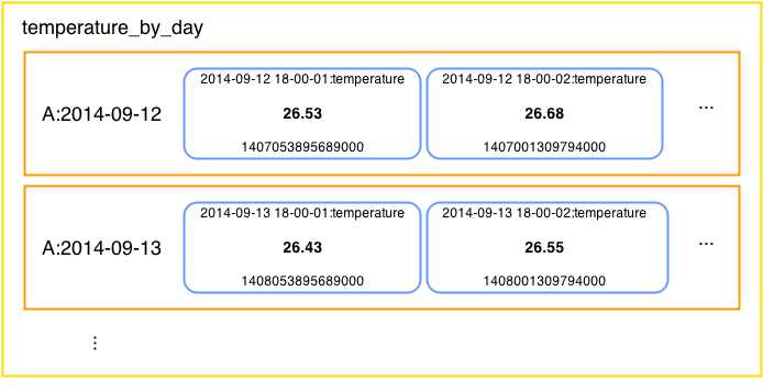
44. Day-level partitions of a single weather station’s data

Getting the data out will not be as easy as it is with the basic example. As shown in the previous figure, the rows of single weather station data are now partitioned by the day the readings were made. To access data from a specific day, we have to specify the day.

Code Listing 92

Column names are a bit longer in this example, so aliases were used in displaying the columns so that the table could fit into the previous code listing. The alias syntax is relatively simple. To change the column names in the output, all you have to do is to specify the AS keyword after the column or function name and then provide the name to be displayed in the table when the results are fetched. As with the basic example, it is possible to navigate through the readings by specifying the boundary measurement times within the partition (a day in our case). The syntax is pretty similar to the basic use case.

Code Listing 93

The examples up to now actually had precision to the seconds level. We used the formatted time stamps to make everything easier to understand. The CQL shell provides an easy way to insert time stamps on the milliseconds level. The numbers that we are going to use are not easily understandable by humans, so it’s advisable to use some kind of converter from seconds and milliseconds to time stamps and vice versa. It’s easy enough to search the Internet for something such as “convert timestamp online”.

We’ll insert a millisecond-level time stamp measurement for weather station B that occurred at “2014-09-12 18:00:00”—that would be a time stamp with a milliseconds value of 1410537600000. Let’s insert three readings one after another.

Code Listing 94

Let’s have a look at the “2014-09-12” partition for weather station B. To access it, we will need to specify the WHERE part of the SELECT to the desired partition.

Code Listing 95

With the current formatting, it might seem as if all of the temperature readings happened at the same point in time. We know for a fact that we inserted the temperatures with spacing of one millisecond between the readings, and we incremented the temperature by a small amount for every temperature reading just so we could identify them later. Cassandra sorts the reading by the measurement time stamp automatically, so the previous listing seems fine from that point of view. Still, we would like to see the milliseconds instead of the time stamp just to make sure the data is actually stored with the time precision that we require.

To do this, we are going to use a little trick. Cassandra handles binary data pretty well; to do so it is equipped with a lot of functions that enable converting any kind of Cassandra native type to its binary representation and converting binary data to any of the basic types. In Cassandra documentation, these functions are often called the blob functions. You may remember that the time stamp in Cassandra is saved as a 64-bit signed integer representing the number of milliseconds that have passed since midnight 1970-01-01. We could convert the time stamp to its binary representation and then this binary representation back to a number as shown in the following example.

Code Listing 96

In the previous example, we took the time stamp column and converted it to a binary value with the timestampAsBlob function. After that, we converted this binary value to an integer and then displayed it in the column t, all with the help of the blobAsBigint function. Knowing the millisecond value of a time stamp is very useful in situations where you are not sure what time stamp value is actually stored in the column.

For instance, if a result does not fall into a queried range when we are making a SELECT statement or something similar, we will wonder why the row is not displayed in the results. If we look at the millisecond level, we might see that the time stamp is actually a couple of milliseconds greater than zero, and because of that it is not falling within the expected range. We could then adjust the query to cover the omitted results or fix the time stamp value on the row. In Cassandra, a lot of things can and will happen one after another, and the default time stamp precision on the seconds level may be inadequate. We will discuss this further in the following section.

Millisecond is a Long Time

As information systems evolve more and more, things start to happen in a smaller and smaller time frame. Nowadays, there are more systems than ever, where hundreds of events occur within the same millisecond. Most of the time, it’s very hard to synchronize information systems’ clocks to a greater precision than a millisecond. So, the majority of devices, components, and systems don’t keep track of the events on a submillisecond level. Even if they did, the timers would probably be in some kind of offset because the clocks probably wouldn’t be perfectly synchronized.

Now imagine that we are using Cassandra to gather measurements that come from multiple devices. While we’re at it, imagine that there are literally thousands of sources sending information to Cassandra, and that the information the sources are generating comes at a millisecond pace. Now what would happen if, let’s say, ten messages come in within the same millisecond?

The initial answer might be that we need to increase the resolution of a clock and then simply make the measurement mechanisms more precise, but remember that the synchronization on a submillisecond level might reveal itself as pretty impractical. If this solution is not possible, then we could perhaps add additional bytes to the time stamp that we are saving and fill the additional bytes with some pseudorandom values so that we could effectively squeeze more events into a single millisecond. In essence, the Cassandra timeuuid type does exactly this. In fact, the timeuuid type can squeeze so much data into the same millisecond that if we did a billion writes per second over a hundred years, we would have just a 50 percent chance of getting a single timeuuid value collision.

Tip: Use the timeuuid type when multiple events occur within the same millisecond.

There are multiple CQL functions that enable us to work with timeuuid more easily:

• now()
• dateOf()
• unixTimestampOf()
• minTimeuuid() and maxTimeuuid()

We will describe how to use these functions through examples. Our weather measurements are not changing every millisecond. To make the examples more practice-oriented, we will use a sample table that monitors high-volume stock exchange trading. Let’s start by defining a new keyspace.

Code Listing 97

Stock ticks usually consist of the transaction price and a time stamp, something like the following example.

Code Listing 98

Now that we have the table with the timeuuid column set up, let’s see how the timeuuid functions are used. Let’s start with inserting the data. The timeuuid has 32 hexadecimal digits in it. It would be very hard for a human to generate these values, so in effect, we wouldn’t even be able to insert the data into tables. To insert the current timeuuid, we use the now function. This function creates a timeuuid with the current time stamp. If we wanted to insert a stock tick, we would do it as shown in the following code listing.

Code Listing 99

To extract the date from a timeuuid, we use the dateOf function.

Code Listing 100

This is an example where every millisecond is very important and we will probably want to extract the exact milliseconds from a timeuuid. To do that, we will use the unixTimestampOf function.

Code Listing 101

Although the millisecond values from the previous listing are not the same because the client I was using couldn’t insert them fast enough, it could easily happen that the millisecond part is exactly the same. When retrieving the results, this would mean that within the same millisecond there could be multiple results. CQL provides two functions that effectively enable us to get all of the data that have the same millisecond time stamp. They are minTimeuuid and maxTimeuuid, and they return minimum and maximum timeuuid value for any given time stamp. For instance, to get all stock ticks in a single second we would use the following query.

Code Listing 102

Summary

This is the longest chapter in the book and we covered many things in it. CQL is the most important way of interacting with Cassandra so we had a lot of everyday usages to cover. We started off by modeling a used car market in the relational world and then examined how Cassandra would handle the same data, and what would be the best practices for using Cassandra to handle the data modeled by the relational approach.

Next, we described how Cassandra is a rather specific storage engine, so we looked closely at how Cassandra physically stores the data. We talked about tables and their properties, and covered Cassandra data types. While explaining these concepts, we covered the common cases in everyday use. We also mentioned that Cassandra has very limited searching capabilities, at least out of the box, so we described indexes and how to use them.

Since Cassandra is often used for time series data, we discussed the time to live (TTL) concept because time series data is usually compacted or assigned an expiration time in most systems. We also looked into handling data on a submillisecond level. CQL and data modeling are at the core of any Cassandra-based application, so this chapter is the most important one in the book.